Here we include the fully fleshed-out notebooks from my git repo DS-for-LA. This is a practical, linear-algebra-first introduction to data science.
- Least Squares Regression: A Linear Algebra Perspective
- QR Decompositions
- Singular Value Decomposition
- Some notes and concerns
- Principal Component Analysis
- Mini Project: Image Denoising with the Truncated SVD
- Modelling 101
- Bibliography
- License
Least Squares Regression: A Linear Algebra Perspective
Introduction
This is meant to be a not entirely comprehensive introduction to Data Science for the Linear Algebraist. There are, of course, many other complicated topics, but this is just to get the essence of data science (and the tools involved) from the perspective of someone with a strong linear algebra background.
One of the most fundamental questions of data science is the following.
Question: Given observed data, how can we predict certain targets?
The answer, of course, boils down to linear algebra, and we will begin by translating data science terms and concepts into linear algebraic ones. But first, as should be common practice for the linear algebraist, an example.
Example. Suppose that we observe $n=3$ houses, and for each house we record
- the square footage,
- the number of bedrooms,
- and the sale price.
So we have a table as follows.
House Square ft Bedrooms Price (in $1000s) 0 1600 3 500 1 2100 4 650 2 1550 2 475 So, for example, the first house is 1600 square feet, has 3 bedrooms, and costs 500,000, and so on. Our goal will be to understand the cost of a house in terms of the number of bedrooms as well as the square footage. Concretely this gives us a matrix and a vector: $$ X = \begin{bmatrix} 1600 & 3 \\ 2100 & 4 \\ 1550 & 2 \end{bmatrix} \text{ and } y =\begin{bmatrix} 500 \\ 650 \\ 475 \end{bmatrix} $$ So translating to linear algebra, the goal is to understand how $y$ depends on the columns of $X$.
Translation from Data Science to Linear Algebra
| Data Science (DS) Term | Linear Algebra (LA) Equivalent | Explanation |
|---|---|---|
| Dataset (with n observations and p features) | A matrix $X \in \mathbb{R}^{n \times p}$ | The dataset is just a matrix. Each row is an observation (a vector of features). Each column is a feature (a vector of its values across all observations). |
| Features | Columns of $X$ | Each feature is a column in your data matrix. |
| Observation | Rows of $X$ | Each data point corresponds to a row. |
| Targets | A vector $y \in \mathbb{R}^{n \times 1}$ | The list of all target values is a column vector. |
| Model parameters | A vector $\beta \in \mathbb{R}^{p \times 1}$ | These are the unknown coefficients. |
| Model | Matrix–vector equation | The relationship becomes an equation involving matrices and vectors. |
| Prediction Error / Residuals | A residual vector $e \in \mathbb{R}^{n \times 1}$ | Difference between actual targets and predictions. |
| Training / “best fit” | Optimization: minimizing the norm of the residual vector | To find the “best” model by finding a model which makes the norm of the residual vector as small as possible. |
So our matrix $X$ will represent our data set, our vector $y$ is the target, and $\beta$ is our vector of parameters. We will often be interested in understanding data with “intercepts”, i.e., when there is a base value given in our data. So we will augment a column of 1’s (denoted by $\mathbb{1}$) to $X$ and append a parameter $\beta_0$ to the top of $\beta$, yielding
$$ \tilde{X} = \begin{bmatrix} \mathbb{1} & X \end{bmatrix} \text{ and } \tilde{\beta} = \begin{bmatrix} \beta_0 \\ \beta_1 \\ \beta_2 \\ \vdots \\ \beta_p \end{bmatrix}. $$
So the answer to the Data Science problem becomes:
Answer: Solve, or best approximate a solution to, the matrix equation $\tilde{X}\tilde{\beta} = y$.
To be explicit, given $\tilde{X}$ and $y$, we want to find a $\tilde{\beta}$ that does a good job of roughly giving $\tilde{X}\tilde{\beta} = y$. There are, of course, ways to solve (or approximate) such small systems by hand. However, one will often be dealing with enormous datasets with plenty of imperfections. One view to take is that modern data science is applying numerical linear algebra techniques to imperfect information, all to get as good a solution as possible.
Solving the problem: Least Squares Regression and Matrix Decompositions
If the system $\tilde{X}\tilde{\beta} = y$ is consistent, then we can find a solution. However, we are often dealing with overdetermined systems, in the sense that there are often more observations than features (i.e., more rows than columns in $\tilde{X}$, or more equations than unknowns), and therefore inconsistent systems. However, it is possible to find a best fit solution, in the sense that the difference
$$ e = y - \tilde{X}\tilde{\beta} $$
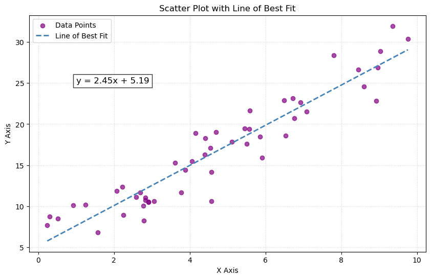
is small. By small, we often mean that $e$ is small in $L^2$ norm; i.e., we are minimizing the sum of the squares of the differences between the components of $y$ and the components of $\tilde{X}\tilde{\beta}$. This is known as a least squares solution. Assuming that our data points live in the Euclidean plane, this precisely describes finding a line of best fit.
import numpy as np
import matplotlib.pyplot as plt

# 1. Generate some synthetic data
# We set a random seed for reproducibility
np.random.seed(3)

# Create 50 random x values between 0 and 10
x = np.random.uniform(0, 10, 50)

# Create y values with a linear relationship plus some random noise
# True relationship: y = 2.5x + 5 + noise
noise = np.random.normal(0, 2, 50)
y = 2.5 * x + 5 + noise

# 2. Calculate the line of best fit
# np.polyfit(x, y, deg) returns the coefficients for the polynomial
# deg=1 specifies a linear fit (first degree polynomial)
slope, intercept = np.polyfit(x, y, 1)

# Create a polynomial function from the coefficients
# This allows us to pass x values directly to get predicted y values
fit_function = np.poly1d((slope, intercept))

# Generate x values for plotting the line (smoothly across the range)
x_line = np.linspace(x.min(), x.max(), 100)
y_line = fit_function(x_line)

# 3. Plot the data and the line of best fit
plt.figure(figsize=(10, 6))

# Plot the scatter points
plt.scatter(x, y, color='purple', label='Data Points', alpha=0.7)

# Plot the line of best fit
plt.plot(x_line, y_line, color='steelblue', linestyle='--', linewidth=2, label='Line of Best Fit')

# Add labels and title
plt.xlabel('X Axis')
plt.ylabel('Y Axis')
plt.title('Scatter Plot with Line of Best Fit')

# Add the equation to the plot
# The f-string formats the slope and intercept to 2 decimal places
plt.text(1, 25, f'y = {slope:.2f}x + {intercept:.2f}', fontsize=12, bbox=dict(facecolor='white', alpha=0.8))

# Display legend and grid
plt.legend()
plt.grid(True, linestyle=':', alpha=0.6)

# Show the plot
plt.savefig('../images/line_of_best_fit_generated_1.png')
plt.show()
The structure of this section is as follows.
Least Squares Solution
Recall that the Euclidean distance between two vectors $x = (x_1,\dots,x_n), y = (y_1,\dots,y_n) \in \mathbb{R}^n$ is given by
$$ \lvert x - y \rvert_2 = \sqrt{\sum_{i=1}^n |x_i - y_i|^2}. $$
We will often work with the square of the $L^2$ norm to simplify things (the square function is increasing, so minimizing the square of a non-negative function will also minimize the function itself).
Definition: Let $A$ be an $m \times n$ matrix and $b \in \mathbb{R}^n$. A least-squares solution of $Ax = b$ is a vector $x_0 \in \mathbb{R}^n$ such that
$$ |b - Ax_0|_2 \leq |b - Ax|_2 \text{ for all } x \in \mathbb{R}^n. $$
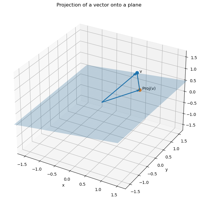
So a least-squares solution to the equation $Ax = b$ is trying to find a vector $x_0 \in \mathbb{R}^n$ which realizes the smallest distance between the vector $b$ and the column space $$ \text{Col}(A) = {Ax \mid x \in \mathbb{R}^n} $$ of $A$. We know this to be the projection of the vector $b$ onto the column space.
import numpy as np
import matplotlib.pyplot as plt

# Linear algebra helper functions
def proj_onto_subspace(A, v):
    """
    Project vector v onto Col(A) where A is (3 x k) with columns spanning the subspace.
    Uses the formula: P = A (A^T A)^(-1) A^T (for full column rank A).
    """
    AtA = A.T @ A
    return A @ np.linalg.solve(AtA, A.T @ v)

def make_plane_grid(a, b, u_range=(-1.5, 1.5), v_range=(-1.5, 1.5), n=15):
    """
    Plane through origin spanned by vectors a and b.
    Returns meshgrid points X,Y,Z for surface plotting.
    """
    uu = np.linspace(*u_range, n)
    vv = np.linspace(*v_range, n)
    U, V = np.meshgrid(uu, vv)
    P = U[..., None] * a + V[..., None] * b   # shape (n,n,3)
    return P[..., 0], P[..., 1], P[..., 2]

# Choose a plan and a vector
# Plane basis vectors (span a 2D subspace in R^3)
a = np.array([1.0, 0.2, 0.0])
b = np.array([0.2, 1.0, 0.3])
# Create the associated matrix
# 3x2 matrix of full column rank
# the column space will be a plane
A = np.column_stack([a, b])

# Vector to project
v = np.array([0.8, 0.6, 1.2])

# Projection and residual
p = proj_onto_subspace(A, v)
r = v - p

# Plot
fig = plt.figure(figsize=(9, 7))
# 1 row, 1 column, 1 subplot
# axis lives in R^3
ax = fig.add_subplot(111, projection="3d")

# Plane surface
X, Y, Z = make_plane_grid(a, b)
# Here is a rectangular grid of points in 3D; draw a surface through them.
ax.plot_surface(X, Y, Z, alpha=0.25)

origin = np.zeros(3)

# v, p, and residual r
ax.quiver(*origin, *v, arrow_length_ratio=0.08, linewidth=2)
ax.quiver(*origin, *p, arrow_length_ratio=0.08, linewidth=2)
ax.quiver(*p, *r, arrow_length_ratio=0.08, linewidth=2)

# Drop line from v to its projection on the plane
ax.plot([v[0], p[0]],
		[v[1], p[1]],
		[v[2], p[2]],
		linestyle="--", linewidth=2)

# Points for emphasis
ax.scatter(*v, s=60)
ax.scatter(*p, s=60)

# Labels (simple text)
ax.text(*v, "  v")
ax.text(*p, "  Proj(v)")

# Make axes look nice
ax.set_xlabel("x")
ax.set_ylabel("y")
ax.set_zlabel("z")
ax.set_title("Projection of a vector onto a plane")

# Set symmetric limits so the picture isn't squished
all_pts = np.vstack([origin, v, p])
m = np.max(np.abs(all_pts)) * 1.3 + 0.2
ax.set_xlim(-m, m)
ax.set_ylim(-m, m)
ax.set_zlim(-m, m)

# Adjust spacing so labels, titles, and axes don’t overlap or get cut off.
plt.tight_layout()
plt.savefig('../images/projection_of_vector_onto_plane.png')
plt.show()
Theorem: The set of least-squares solutions of $Ax = b$ coincides with solutions of the normal equations $A^TAx = A^Tb$. Moreover, the normal equations always have a solution.
Let us first see why we get a line of best fit.
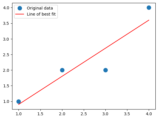
Example. Let us show why this describes a line of best fit when we are working with one feature and one target. Suppose that we observe four data points $$ X = \begin{bmatrix} 1 \\ 2 \\ 3 \\ 4 \end{bmatrix} \text{ and } y = \begin{bmatrix} 1 \\ 2\\ 2 \\ 4 \end{bmatrix}. $$ We want to fit a line $y = \beta_0 + \beta_1x$ to these data points. We will have our augmented matrix be $$ \tilde{X} = \begin{bmatrix} 1 & 1 \\ 1 & 2 \\ 1 & 3 \\ 1 & 4 \end{bmatrix}, $$ and our parameter be $$ \tilde{\beta} = \begin{bmatrix} \beta_0 \\ \beta_1 \end{bmatrix}. $$ We have that $$ \tilde{X}^T\tilde{X} = \begin{bmatrix} 4 & 10 \\ 10 & 30 \end{bmatrix} \text{ and } \tilde{X}^Ty = \begin{bmatrix} 9 \\ 27 \end{bmatrix}. $$ The 2x2 matrix $\tilde{X}^T\tilde{X}$ is easy to invert, and so we get that $$ \tilde{\beta} = (\tilde{X}^T\tilde{X})^{-1}\tilde{X}^Ty = \frac{1}{10}\begin{bmatrix} 15 & -5 \\ -5 & 2 \end{bmatrix}\begin{bmatrix} 9 \\ 27 \end{bmatrix} = \begin{bmatrix} 0 \\ \frac{9}{10} \end{bmatrix}. $$ So our line of best fit is of the form $y = \frac{9}{10}x$.
Although the above system was small and we could solve the system of equations explicitly, this isn’t always feasible. We will generally use Python in order to solve large systems.
- One can find a least-squares solution using
numpy.linalg.lstsq. - We can set up the normal equations and solve the system by using
numpy.linalg.solve. Although the first approach simplifies things greatly, and is more or less what we are doing anyway, we will generally set up our problems as we would by hand, and then usenumpy.linalg.solveto help us find a solution. However, computing $X^TX$ can cause lots of errors, so later we’ll see how to get linear systems from QR decompositions and the SVD, and then applynumpy.linalg.solve.
Let’s see how to use these for the above example, and see the code to generate the scatter plot and line of best fit. Again, our system is the following. $$ X = \begin{bmatrix} 1 \\ 2 \\ 3 \\ 4 \end{bmatrix} \text{ and } y = \begin{bmatrix} 1 \\ 2\\ 2 \\ 4 \end{bmatrix}. $$ We will do what we did above, but use Python instead.
import numpy as np

# Define the matrix X and vector y
X = np.array([[1], [2], [3], [4]])
y = np.array([[1], [2], [2], [4]])

# Augment X with a column of 1's (intercept)
X_aug = np.hstack((np.ones((X.shape[0], 1)), X))

# Solve the normal equations
beta = np.linalg.solve(X_aug.T @ X_aug, X_aug.T @ y)
And what is the result?
beta
array([[-1.0658141e-15],
       [ 9.0000000e-01]])
This agrees with our by-hand computation: the intercept is tiny, so it is virtually zero, and we get 9/10 as our slope. Let’s plot it.
import matplotlib.pyplot as plt
b, m  = beta #beta[0] will be the intercept and beta[1] will be the slope
_ = plt.plot(X, y, 'o', label='Original data', markersize=10)
_ = plt.plot(X, m*X + b, 'r', label='Line of best fit')
_ = plt.legend()
plt.savefig('../images/line_of_best_fit_easy_example.png')
plt.show()
What about numpy.linalg.lstsq? Is it any different?
import numpy as np

# Define the matrix X and vector y
X = np.array([[1], [2], [3], [4]])
y = np.array([[1], [2], [2], [4]])

# Augment X with a column of 1's (intercept)
X_aug = np.hstack((np.ones((X.shape[0], 1)), X))

# Solve the least squares equation with matrix X_aug and target y
beta = np.linalg.lstsq(X_aug,y)[0]
We then get
beta
array([[6.16291085e-16],
       [9.00000000e-01]])
So it is a little different – and, in fact, closer to our exact answer (the intercept is zero). This makes sense – numpy.linalg.lstsq won’t directly compute $X^TX$, which, again, can cause quite a few issues.
Now, going back to our initial example.
Example: Let us work with the example from above. We augment the matrix with a column of 1’s to include an intercept term: $$ \tilde{X} = \begin{bmatrix} 1 & 1600 & 3 \\ 1 & 2100 & 4 \\ 1 & 1550 & 2 \end{bmatrix}. $$ Let us solve the normal equations $$ \tilde{X}^T\tilde{X}\tilde{\beta} = \tilde{X}^Ty. $$ We have $$ \tilde{X}^T\tilde{X} = \begin{bmatrix} 3 & 5250 & 9 \\ 5250 & 9372500 & 16300 \\ 9 & 16300 & 29\end{bmatrix} \text{ and } \tilde{X}^Ty = \begin{bmatrix} 1625 \\ 2901500 \\ 5050 \end{bmatrix} $$ Solving this system of equations yields the parameter vector $\tilde{\beta}$. In this case, we have $$ \tilde{\beta} = \begin{bmatrix} \frac{200}{9} \\ \frac{5}{18} \\ \frac{100}{9} \end{bmatrix}. $$ When we apply $\tilde{X}$ to $\tilde{\beta}$, we get $$ \tilde{X}\tilde{\beta} = \begin{bmatrix} 500 \\ 650 \\ 475 \end{bmatrix}, $$ which is our target on the nose. This means that we can expect, based on our data, that the cost of a house will be $$ \frac{200}{9} + \frac{5}{18}(\text{square footage}) + \frac{100}{9}(\text{\# of bedrooms})$$
In the above, we actually had a consistent system to begin with, so our least-squares solution gave our prediction honestly. What happens if we have an inconsistent system?
Example: Let us add two more observations, say our data is now the following.
House Square ft Bedrooms Price (in $1000s) 0 1600 3 500 1 2100 4 650 2 1550 2 475 3 1600 3 490 4 2000 4 620 So setting up our system, we want a least-square solution to the matrix equation $$ \begin{bmatrix} 1 & 1600 & 3 \\ 1 & 2100 & 4 \\ 1 & 1550 & 2 \\ 1 & 1600 & 3 \\ 1 & 2000 & 4 \end{bmatrix}\tilde{\beta} = \begin{bmatrix} 500 \\ 650 \\ 475 \\ 490 \\ 620 \end{bmatrix}. $$ Note that the system is inconsistent (the 1st and 4th rows agree in $\tilde{X}$, but they have different costs). Writing the normal equations we have $$ \tilde{X}^T\tilde{X} = \begin{bmatrix} 5 & 8850 & 16 \\ 8850 & 15932500 & 29100 \\ 16 & 29100 & 54 \end{bmatrix} \text{ and } \tilde{X}^Ty = \begin{bmatrix} 2735 \\ 4,925,250 \\ 9000 \end{bmatrix}. $$ Solving this linear system yields $$ \tilde{\beta} = \begin{bmatrix} 0 \\ \frac{3}{10} \\ 5 \end{bmatrix}. $$ This is a vastly different answer! Applying $\tilde{X}$ to it yields $$ \tilde{X}\tilde{\beta} = \begin{bmatrix} 495 \\ 650 \\ 475 \\ 495 \\ 620 \end{bmatrix}. $$ Note that the error here is $$ y - \tilde{X}\tilde{\beta} = \begin{bmatrix} 5 \\ 0 \\ 0 \\ -5 \\ 0 \end{bmatrix}, $$ which has squared $L^2$ norm $$ |y - \tilde{X}\tilde{\beta}|_2^2 = 25 + 25 = 50. $$ So this says that, given our data, we can roughly estimate the cost of a house, within 50k or so, to be $$ \approx \frac{3}{10}(\text{square footage}) + 5(\text{\# of bedrooms}). $$ In practice, our data sets can be gigantic, and so there is absolutely no hope of doing computations by hand. It is nice to know that theoretically we can do things like this though.
Theorem: Let $A$ be an $m \times n$ matrix and $b \in \mathbb{R}^n$. The following are equivalent.
- The equation $Ax = b$ has a unique least-squares solution for each $b \in \mathbb{R}^n$.
- The columns of $A$ are linearly independent.
- The matrix $A^TA$ is invertible.
In this case, the unique solution to the normal equations $A^TAx = A^Tb$ is
$$ x_0 = (A^TA)^{-1}A^Tb. $$
Computing $\tilde{X}^T\tilde{X}$ or taking inverses are very computationally intensive tasks, and it is best to avoid doing these. Moreover, as we’ll see in an example later, if we do a numerical calculation we can get close to zero and then divide where we shouldn’t be, blowing up our final result. One way to get around this is to use QR decompositions of matrices.
Now let’s use Python to visualize the above data and then solve for the least-squares solution. We’ll use pandas in order to think about this data. We note that pandas incorporates matplotlib under the hood already, so there are some simplifications that can be made.
import numpy as np
import pandas as pd
import matplotlib.pyplot as plt

# First let us make a dictionary incorporating our data.
# Each entry corresponds to a column (feature of our data)
data = {
	'Square ft': [1600, 2100, 1550, 1600, 2000],
	'Bedrooms': [3, 4, 2, 3, 4],
	'Price': [500, 650, 475, 490, 620]
}

# Create a pandas DataFrame
df = pd.DataFrame(data)
Let’s see how Python formats this DataFrame. It will turn it into essentially the table we had at the beginning.
df
| Square ft | Bedrooms | Price | |
|---|---|---|---|
| 0 | 1600 | 3 | 500 |
| 1 | 2100 | 4 | 650 |
| 2 | 1550 | 2 | 475 |
| 3 | 1600 | 3 | 490 |
| 4 | 2000 | 4 | 620 |
So what can we do with DataFrames? First let’s use pandas.DataFrame.describe to see some basic statistics about our data.
df.describe()
| Square ft | Bedrooms | Price | |
|---|---|---|---|
| count | 5.000000 | 5.00000 | 5.000000 |
| mean | 1770.000000 | 3.20000 | 547.000000 |
| std | 258.843582 | 0.83666 | 81.516869 |
| min | 1550.000000 | 2.00000 | 475.000000 |
| 25% | 1600.000000 | 3.00000 | 490.000000 |
| 50% | 1600.000000 | 3.00000 | 500.000000 |
| 75% | 2000.000000 | 4.00000 | 620.000000 |
| max | 2100.000000 | 4.00000 | 650.000000 |
This gives us the mean, the standard deviation, the min, the max, as well as some other things. We get an immediate sense of scale from our data. We can also examine the pairwise correlation of all the columns by using pandas.DataFrame.corr.
df[["Square ft", "Bedrooms", "Price"]].corr()
| Square ft | Bedrooms | Price | |
|---|---|---|---|
| Square ft | 1.000000 | 0.900426 | 0.998810 |
| Bedrooms | 0.900426 | 1.000000 | 0.909066 |
| Price | 0.998810 | 0.909066 | 1.000000 |
It is clear that all three are correlated. This makes sense, as the number of bedrooms should increase with square footage, as should the price. We’ll discuss this in the next section when we look at Principal Component Analysis.
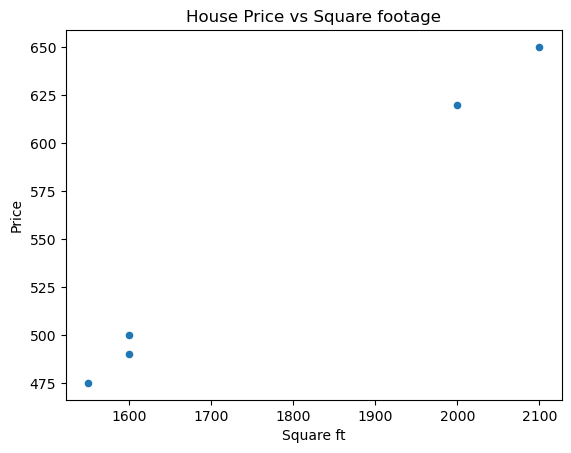
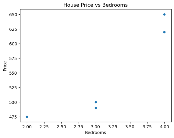
We can also graph our data; for example, we could create some scatter plots, one for Square ft vs Price and one for Bedrooms vs Price. We can also do a grouped bar chart. Let’s start with the scatter plots.
# Scatter plot for Price vs Square ft
df.plot(
	kind="scatter",
	x="Square ft",
	y="Price",
	title="House Price vs Square footage"
)
plt.savefig('../images/house_price_vs_square_ft.png')
plt.show()
# Scatter plot for Price vs Bedrooms
df.plot(
	kind="scatter",
	x="Bedrooms",
	y="Price",
	title="House Price vs Bedrooms"
)
plt.savefig('../images/house_price_vs_bedrooms.png')
plt.show()
We can even do square footage vs bedrooms.
# Scatter plot for Bedrooms vs Square ft
df.plot(
	kind="scatter",
	x="Square ft",
	y="Bedrooms",
	title="Bedrooms vs Square footage"
)
plt.savefig('../images/bedrooms_vs_square_ft.png')
plt.show()
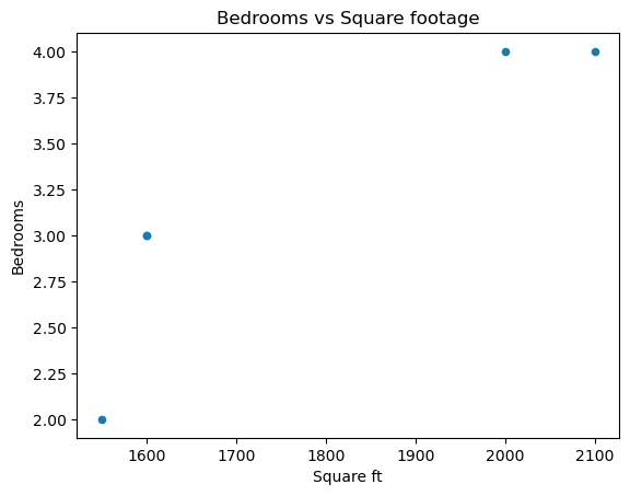
Of course, these figures are somewhat meaningless due to how unpopulated our data is.
Now let’s get our matrices and linear systems set up with pandas.DataFrame.to_numpy.
# Create our matrix X and our target y
X = df[["Square ft", "Bedrooms"]].to_numpy()
y = df[["Price"]].to_numpy()

# Augment X with a column of 1's (intercept)
X_aug = np.hstack((np.ones((X.shape[0], 1)), X))

# Solve the least-squares problem
beta = np.linalg.lstsq(X_aug,y)[0]
This yields
beta
array([[4.0098513e-13],
       [3.0000000e-01],
       [5.0000000e+00]])
As the first parameter is basically 0, we are left with the second being 3/10 and the third being 5, just like our exact solution. Next, we will look at matrix decompositions and how they can help us find least-squares solutions.
Polynomial Regression
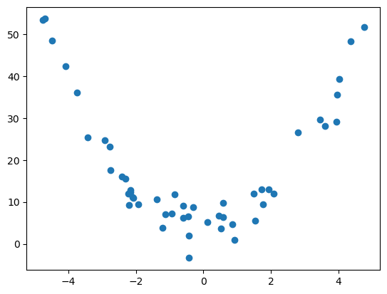
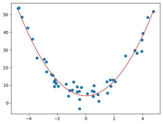
Sometimes fitting a line to a set of $n$ data points clearly isn’t the right thing to do. To emphasize the limitations of linear models, we generate data from a purely quadratic relationship. In this setting, the space of linear functions is not rich enough to capture the underlying structure, and the linear least-squares solution exhibits systematic error. Expanding the feature space to include quadratic terms resolves this issue.
For example, suppose our data looked like the following.
## Generate data
import numpy as np
import matplotlib.pyplot as plt

# 1) Generate quadratic data
np.random.seed(3)

n = 50
x = np.random.uniform(-5, 5, n)   # symmetric, wider range

# True relationship: y = ax^2 + c + noise
a_true = 2.0
c_true = 5.0
noise = np.random.normal(0, 3, n)

y = a_true * x**2 + c_true + noise

## Generate scatter plot
plt.scatter(x,y)

# plot it
plt.savefig('../images/quadratic_data_generated_1.png')
plt.show()
If we try to find a line of best fit, we get something that doesn’t really describe or approximate our data at all…
# find a line of best fit
a,b = np.polyfit(x, y, 1)

# add scatter points to plot
plt.scatter(x,y)

# add line of best fit to plot
plt.plot(x, a*x + b, 'r', linewidth=1)

# plot it
plt.savefig('../images/quadratic_data_line_of_best_fit.png')
plt.show()
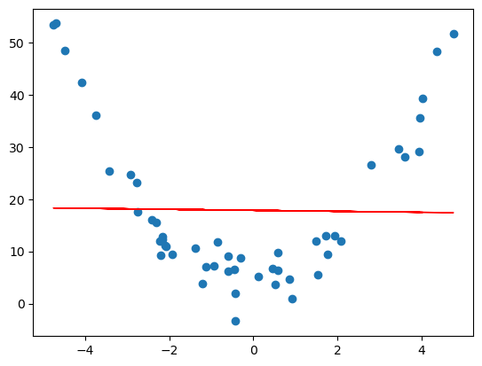
This is an example of underfitting data, and we can do better. The same linear regression ideas work for fitting a degree $d$ polynomial model to a set of $n$ data points. Before, when trying to fit a line to points $(x_1,y_1),\dots,(x_n,y_n)$, we had the following matrices $$ \tilde{X} = \begin{bmatrix} 1 & x_1 \\ \vdots & \vdots \\ 1 & x_n \end{bmatrix}, y = \begin{bmatrix} y_1 \\ \vdots \\ y_n \end{bmatrix}, \tilde{\beta} = \begin{bmatrix} \beta_0 \\ \beta_1 \end{bmatrix} $$ in the matrix equation $$ \tilde{X}\tilde{\beta} = y, $$ and we were trying to find a vector $\tilde{\beta}$ which gave a best possible solution. This would give us a line $y = \beta_0 + \beta_1x$ which best approximates the data. To fit a polynomial $y = \beta_0 + \beta_1x + \beta_2x^2 + \cdots + \beta_dx^d$ to the data, we have a similar set up.
Definition. The Vandermonde matrix is the $n \times (d+1)$ matrix $$ V = \begin{bmatrix} 1 & x_1 & x_1^2 & \cdots & x_1^d \\ 1 & x_2 & x_2^2 & \cdots & x_2^d \\ \vdots & \vdots & \ddots & \vdots \\ 1 & x_n & x_n^2 & \cdots & x_n^d \end{bmatrix}. $$
With the Vandermonde matrix, to find a polynomial function of best fit, one just needs to find a least-squares solution to the matrix equation $$ V\tilde{\beta} = y. $$
With the generated data above, we get the following curve.
# polynomial fit with degree = 2
poly = np.polyfit(x,y,2)
model = np.poly1d(poly)

# add scatter points to plot
plt.scatter(x,y)

# add the quadratic to the plot
polyline=np.linspace(x.min(), x.max())
plt.plot(polyline, model(polyline), 'r', linewidth=1)


# plot it
plt.savefig('../images/quadratic_data_quadratic_of_best_fit')
plt.show()
Solving these problems can be done with Python. One can use numpy.polyfit and numpy.poly1d.
Example. Consider the following data.
House Square ft Bedrooms Price (in $1000s) 0 1600 3 500 1 2100 4 650 2 1550 2 475 3 1600 3 490 4 2000 4 620 Suppose we wanted to predict the price of a house based on the square footage and we thought the relationship was cubic (it clearly isn’t, but hey, for the sake of argument). So really we are looking at the subset of data
House Square ft Price (in $1000s) 0 1600 500 1 2100 650 2 1550 475 3 1600 490 4 2000 620 Our Vandermonde matrix will be $$ V = \begin{bmatrix} 1 & 1600 & 1600^2 & 1600^3 \\ 1 & 2100 & 2100^2 & 2100^3 \\ 1 & 1550 & 1550^2 & 1550^3 \\ 1 & 1600 & 1600^2 & 1600^3 \\ 1 & 2000 & 2000^2 & 2000^3 \end{bmatrix} $$ and our target vector will be $$ y = \begin{bmatrix} 500 \\ 650 \\ 475 \\ 490 \\ 620 \end{bmatrix}. $$ As we can see, the entries of the Vandermonde matrix get very very large very fast. One can, if they are so inclined, compute a least-squares solution to $V\tilde{\beta} = y$ by hand. Let’s not, but let us find, using Python, a “best” cubic approximation of the relationship between the square footage and price.
We will use numpy.polyfit, numpy.poly1d and numpy.linspace.
Let’s get a cubic of best fit.
import numpy as np
import pandas as pd
import matplotlib.pyplot as plt

# First let us make a dictionary incorporating our data.
# Each entry corresponds to a column (feature of our data)
data = {
    'Square ft': [1600, 2100, 1550, 1600, 2000],
    'Bedrooms': [3, 4, 2, 3, 4],
    'Price': [500, 650, 475, 490, 620]
}

# Create a pandas DataFrame
df = pd.DataFrame(data)

# Extract x (square footage) and y (price)
x = df["Square ft"].to_numpy(dtype=float)
y = df["Price"].to_numpy(dtype=float)

# Degree of polynomial
degree = 3 # cubic

# Polyfit directly on x
cubic = np.poly1d(np.polyfit(x,y, degree))

# Add fitted polynomial line and scatter plot
polyline = np.linspace(x.min(),x.max())
plt.scatter(x,y, label="Observed data")
plt.plot(polyline, cubic(polyline), 'r', label="Cubic best fit")
plt.xlabel("Square ft")
plt.ylabel("Price (in $1000s)")
plt.title("Cubic polynomial regression: Price vs Square Footage")
plt.show()
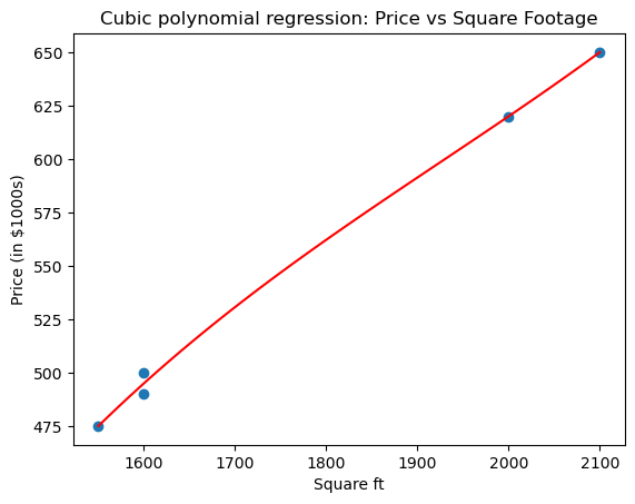
Here numpy.polyfit computes the least-squares solution in the polynomial basis $1, x, x^2, x^3$, i.e., it solves the Vandermonde least-squares problem. So what is our cubic polynomial?
cubic
poly1d([ 3.08080808e-07, -1.78106061e-03, 3.71744949e+00, -2.15530303e+03])
The first term is the degree 3 term, the second the degree 2 term, the third the degree 1 term, and the fourth is the constant term.
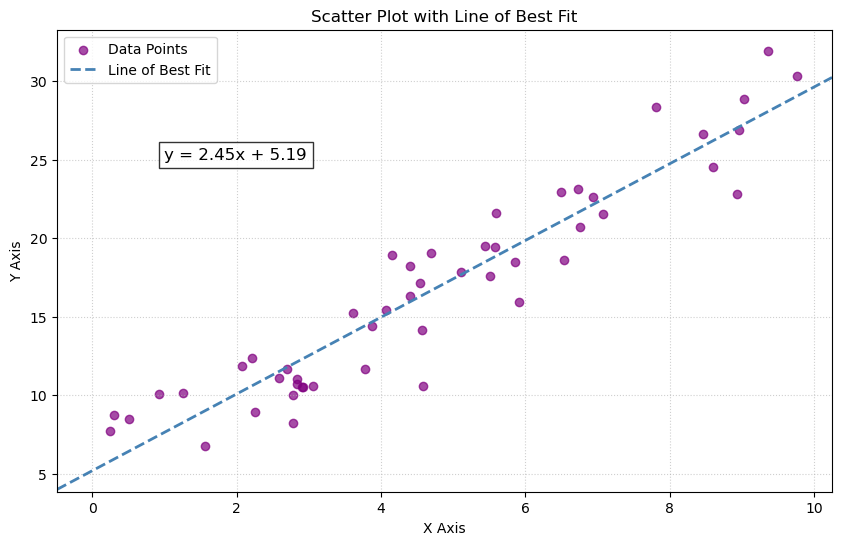
Additional visualization: line of best fit
The first figure is a line of best fit for scattered points. Here is some alternate code that will produce an image. We can do the following using matplotlib.pyplot.axline.
import numpy as np
import matplotlib.pyplot as plt

# Generate data (same as above)
np.random.seed(3)
x = np.random.uniform(0, 10, 50)
y = 2.5 * x + 5 + np.random.normal(0, 2, 50)

# Calculate slope and intercept
slope, intercept = np.polyfit(x, y, 1)

plt.figure(figsize=(10, 6))
plt.scatter(x, y, color='purple', label='Data Points', alpha=0.7)
# Plot the line using axline
# xy1=(0, intercept) is the y-intercept point

# slope=slope defines the steepness
plt.axline(xy1=(0, intercept), slope=slope, color='steelblue', linestyle='--', linewidth=2, label='Line of Best Fit')

# Add the equation to the plot
# The f-string formats the slope and intercept to 2 decimal places
plt.text(1, 25, f'y = {slope:.2f}x + {intercept:.2f}', fontsize=12, bbox=dict(facecolor='white', alpha=0.8))


plt.xlabel('X Axis')
plt.ylabel('Y Axis')
plt.title('Scatter Plot with Line of Best Fit')
plt.legend()
plt.grid(True, linestyle=':', alpha=0.6)
plt.show()
See
- https://stackoverflow.com/questions/37234163/how-to-add-a-line-of-best-fit-to-scatter-plot
- https://www.statology.org/line-of-best-fit-python/
- https://stackoverflow.com/questions/6148207/linear-regression-with-matplotlib-numpy
QR Decompositions
QR decompositions are a powerful tool in linear algebra and data science for several reasons. They provide a way to decompose a matrix into an orthogonal matrix $Q$ and an upper triangular matrix $R$, which can simplify many computations and analyses.
Theorem: Let $A$ be an $m \times n$ matrix with linearly independent columns ($m \geq n$ in this case). Then $A$ can be decomposed as $A = QR$ where $Q$ is an $m \times n$ matrix whose columns form an orthonormal basis for Col($A$) and $R$ is an $n \times n$ upper-triangular invertible matrix with positive entries on the diagonal.
In the literature, sometimes the QR decomposition is phrased as follows: any $m \times n$ matrix $A$ can also be written as $A = QR$ where $Q$ is an $m \times m$ orthogonal matrix ($Q^T = Q^{-1}$), and $R$ is an $m \times n$ upper-triangular matrix. One follows from the other by playing around with some matrix equations. Indeed, suppose that $A = Q_1R_1$ is a decomposition as above (that is, $Q_1$ is $m \times n$ and $R_1$ is $n \times n$). One can use the Gram-Schmidt procedure to extend the columns of $Q_1$ to an orthonormal basis for all of $\mathbb{R}^m$, and put the remaining vectors in an $m \times (m - n)$ matrix $Q_2$. Then
$$ A = Q_1R_1 = \begin{bmatrix} Q_1 & Q_2 \end{bmatrix}\begin{bmatrix} R_1 \\ 0 \end{bmatrix}. $$
The left matrix is an $m \times m$ orthogonal matrix and the right matrix is $m \times n$ upper triangular. Moreover, the decomposition provides orthonormal bases for both the column space of $A$ and the perp of the column space of $A$; $Q_1$ will consist of an orthonormal basis for the column space of $A$ and $Q_2$ will consist of an orthonormal basis for the perp of the column space of $A$.
However, we will often want to use the decomposition when $Q$ is $m \times n$, $R$ is $n \times n$, and the columns of $Q$ form an orthonormal basis for the column space of $A$. For example, the Python function numpy.linalg.qr gives QR decompositions this way (again, assuming that the columns of $A$ are linearly independent, so $m \geq n$).
Key take-away. The QR decomposition provides an orthonormal basis for the column space of $A$. If $A$ has rank $k$, then the first $k$ columns of $Q$ will form a basis for the column space of $A$.
For small matrices, one can find $Q$ and $R$ by hand, assuming that $A = [ a_1\ \cdots\ a_n ]$ has full column rank. Let $e_1,\dots,e_n$ be the unnormalized vectors we get when we apply Gram-Schmidt to $c_1,\dots,c_n$, and let $u_1,\dots,u_n$ be their normalizations. Let $$ r_j = \begin{bmatrix} \langle e_1,c_j \rangle \\ \vdots \\ \langle e_n, c_j \rangle \end{bmatrix}, $$ and note that $\langle e_i,c_j \rangle = 0$ whenever $i > j$. Thus $$ Q = \begin{bmatrix} u_1 & \cdots & u_n \end{bmatrix} \text{ and } R = \begin{bmatrix} r_1 & \cdots & r_n \end{bmatrix} $$ give rise to a $A = QR$, where the columns of $Q$ form an orthonormal basis for $\text{Col}(A)$ and $R$ is upper-triangular. We can also compute $R$ directly from $Q$ and $A$. Indeed, note that $Q^TQ = I$, so $$ Q^TA = Q^T(QR) = IR = R. $$
Example. Find a QR decomposition for the matrix $$ A = \begin{bmatrix} 1 & 1 & 1 \\ 0 & 1 & 1 \\ 0 & 0 & 1 \\ 0 & 0 & 0 \end{bmatrix}. $$ Note that one can trivially see (or by applying the Gram-Schmidt procedure) that $$ \begin{bmatrix} 1 \\ 0 \\ 0 \\ 0 \end{bmatrix}, \begin{bmatrix} 0 \\ 1 \\ 0 \\ 0 \end{bmatrix}, \begin{bmatrix} 0 \\ 0 \\ 1 \\ 0 \end{bmatrix} $$ forms an orthonormal basis for the column space of $A$. So with $$ Q = \begin{bmatrix} 1 & 0 & 0 \\ 0 & 1 & 0 \\ 0 & 0 & 1 \\ 0 & 0 & 0 \end{bmatrix} \text{ and }R = \begin{bmatrix} 1 & 1 & 1\\ 0 & 1 & 1 \\ 0 & 0 & 1 \end{bmatrix}, $$ we have $A = QR$.
Let’s do a more involved example.
Example. Consider the matrix $$ A = \begin{bmatrix} 1 & 0 & 0 \\ 1 & 1 & 0 \\ 1 & 1 & 1 \\ 1 & 1 & 1 \end{bmatrix}. $$ One can apply the Gram-Schmidt procedure to the columns of $A$ to find that $$ \begin{bmatrix} 1 \\ 1 \\ 1 \\ 1 \end{bmatrix}, \begin{bmatrix} -3 \\ 1 \\ 1 \\ 1 \end{bmatrix}, \begin{bmatrix} 0 \\ -\frac{2}{3} \\ \frac{1}{3} \\ \frac{1}{3}\end{bmatrix} $$ forms an orthogonal basis for the column space of $A$. Normalizing, we get that $$ Q = \begin{bmatrix} \frac{1}{2} & -\frac{3}{\sqrt{12}} & 0 \\ \frac{1}{2} & \frac{1}{\sqrt{12}} & -\frac{2}{\sqrt{6}} \\ \frac{1}{2} & \frac{1}{\sqrt{12}} & \frac{1}{\sqrt{6}} \\ \frac{1}{2} & \frac{1}{\sqrt{12}} & \frac{1}{\sqrt{6}} \end{bmatrix} $$ is an appropriate $Q$. Thus $$ \begin{split} R = Q^TA &= \begin{bmatrix} \frac{1}{2} & \frac{1}{2} & \frac{1}{2} & \frac{1}{2} \\ -\frac{3}{\sqrt{12}} & \frac{1}{\sqrt{12}} & \frac{1}{\sqrt{12}} & \frac{1}{\sqrt{12}} \\ 0 & -\frac{2}{\sqrt{6}} & \frac{1}{\sqrt{6}} & \frac{1}{\sqrt{6}} \end{bmatrix}\begin{bmatrix} 1 & 0 & 0 \\ 1 & 1 & 0 \\ 1 & 1 & 1 \\ 1 & 1 & 1 \end{bmatrix} \\ &= \begin{bmatrix} 2 & \frac{3}{2} & 1 \\ 0 & \frac{3}{\sqrt{12}} & \frac{2}{\sqrt{12}} \\ 0 & 0 & \frac{2}{\sqrt{6}} \end{bmatrix}. \end{split} $$ So all together, $$A = \begin{bmatrix} \frac{1}{2} & -\frac{3}{\sqrt{12}} & 0 \\ \frac{1}{2} & \frac{1}{\sqrt{12}} & -\frac{2}{\sqrt{6}} \\ \frac{1}{2} & \frac{1}{\sqrt{12}} & \frac{1}{\sqrt{6}} \\ \frac{1}{2} & \frac{1}{\sqrt{12}} & \frac{1}{\sqrt{6}} \end{bmatrix}\begin{bmatrix} 2 & \frac{3}{2} & 1 \\ 0 & \frac{3}{\sqrt{12}} & \frac{2}{\sqrt{12}} \\ 0 & 0 & \frac{2}{\sqrt{6}} \end{bmatrix}. $$
To do this numerically, we can use numpy.linalg.qr.
import numpy as np

# Define our matrices
A = np.array([[1,1,1],[0,1,1],[0,0,1],[0,0,0]])
B = np.array([[1,0,0],[1,1,0],[1,1,1],[1,1,1]])

# Take QR decompositions
QA, RA = np.linalg.qr(A)
QB, RB = np.linalg.qr(B)
Our resulting matrices are:
print(f"QA = {QA}\n")
print(f"RA = {RA}\n")
print(f"QB = {QB}\n")
print(f"RB = {RB}")
QA = [[ 1.  0.  0.]
 [-0.  1.  0.]
 [-0. -0.  1.]
 [-0. -0. -0.]]

RA = [[1. 1. 1.]
 [0. 1. 1.]
 [0. 0. 1.]]

QB = [[-0.5         0.8660254   0.        ]
 [-0.5        -0.28867513  0.81649658]
 [-0.5        -0.28867513 -0.40824829]
 [-0.5        -0.28867513 -0.40824829]]

RB = [[-2.         -1.5        -1.        ]
 [ 0.         -0.8660254  -0.57735027]
 [ 0.          0.         -0.81649658]]
How to use QR decompositions
One of the primary uses of QR decompositions is to solve least squares problems, as introduced above. Assuming that $A$ has full column rank, we can write $A = QR$ as a QR decomposition, and then we can find a least-squares solution to $Ax = b$ by solving the upper-triangular system.
Theorem. Let $A$ be an $m \times n$ matrix with full column rank, and let $A = QR$ be a QR factorization of $A$. Then, for each $b \in \mathbb{R}^m$, the equation $Ax = b$ has a unique least-squares solution, arising from the system $$ Rx = Q^Tb. $$
Normal equations can be ill-conditioned, i.e., small errors in calculating $A^TA$ give large errors when trying to solve the least-squares problem. When $A$ has full column rank, a QR factorization will allow one to compute a solution to the least-squares problem more reliably.
Example. Let $$ A = \begin{bmatrix} 1 & 0 & 0 \\ 1 & 1 & 0 \\ 1 & 1 & 1 \\ 1 & 1 & 1 \end{bmatrix} \text{ and } b = \begin{bmatrix} 1 \\ 1 \\ 1 \\ 0 \end{bmatrix}. $$ We can find the least-squares solution $Ax = b$ by using the QR decomposition. Let us use the QR decomposition from above, and solve the system $$ Rx = Q^Tb. $$ As $$ \begin{bmatrix} \frac{1}{2} & -\frac{3}{\sqrt{12}} & 0 \\ \frac{1}{2} & \frac{1}{\sqrt{12}} & -\frac{2}{\sqrt{6}} \\ \frac{1}{2} & \frac{1}{\sqrt{12}} & \frac{1}{\sqrt{6}} \\ \frac{1}{2} & \frac{1}{\sqrt{12}} & \frac{1}{\sqrt{6}} \end{bmatrix}^T\begin{bmatrix} 1 \\ 1 \\ 1 \\ 0 \end{bmatrix} = \begin{bmatrix} \frac{3}{2} \\ -\frac{1}{2\sqrt{3}} \\ -\frac{1}{\sqrt{6}}, \end{bmatrix} $$ we are looking at the system $$ \begin{bmatrix} 2 & \frac{3}{2} & 1 \\ 0 & \frac{3}{\sqrt{12}} & \frac{2}{\sqrt{12}} \\ 0 & 0 & \frac{2}{\sqrt{6}} \end{bmatrix}x =\begin{bmatrix} \frac{3}{2} \\ -\frac{1}{2\sqrt{3}} \\ -\frac{1}{\sqrt{6}} \end{bmatrix}. $$ Solving this system yields that $$ x_0 = \begin{bmatrix} 1 \\ 0 \\ -\frac{1}{2} \end{bmatrix} $$ is a least-squares solution to $Ax = b$.
Let us set this system up in Python and use numpy.linalg.solve.
import numpy as np

# Define matrix and vector
A = np.array([[1,0,0],[1,1,0],[1,1,1],[1,1,1]])
b = np.array([[1],[1],[1],[0]])

# Take the QR decomposition of A
Q, R = np.linalg.qr(A)

# Solve the linear system Rx = Q.T b
beta = np.linalg.solve(R,Q.T @ b)
This yields
beta
array([[ 1.00000000e+00],
       [ 6.40987562e-17],
       [-5.00000000e-01]])
which (basically) agrees with our exact least-squares solution.
Note that numpy.linalg.lstsq still gives an ever-so-slightly different result.
np.linalg.lstsq(A,b)[0]
array([[ 1.00000000e+00],
       [ 2.22044605e-16],
       [-5.00000000e-01]])
Let’s go back to the house example. While we’re at it, let’s get used to using pandas to make a dataframe.
import numpy as np
import pandas as pd

# First let us make a dictionary incorporating our data.
# Each entry corresponds to a column (feature of our data)
data = {
    'Square ft': [1600, 2100, 1550, 1600, 2000],
    'Bedrooms': [3, 4, 2, 3, 4],
    'Price': [500, 650, 475, 490, 620]
}

# Create a pandas DataFrame
df = pd.DataFrame(data)

# Create our matrix X and our target y
X = df[["Square ft", "Bedrooms"]].to_numpy()
y = df[["Price"]].to_numpy()

# Augment X with a column of 1's (intercept)
X_aug = np.hstack((np.ones((X.shape[0], 1)), X))

# Perform QR decomposition
Q, R = np.linalg.qr(X_aug)

# Solve the upper triangular system Rx = Q^Ty
beta = np.linalg.solve(R, Q.T @ y)
Let’s look at the output.
print(f"Q = {Q} \n\nR = {R} \n\nbeta = {beta}")
Q = [[-0.4472136   0.32838365  0.40496317]
 [-0.4472136  -0.63745061 -0.22042299]
 [-0.4472136   0.42496708 -0.7689174 ]
 [-0.4472136   0.32838365  0.40496317]
 [-0.4472136  -0.44428376  0.17941406]]

R = [[-2.23606798e+00 -3.95784032e+03 -7.15541753e+00]
 [ 0.00000000e+00 -5.17687164e+02 -1.50670145e+00]
 [ 0.00000000e+00  0.00000000e+00  7.27908474e-01]]

beta = [[-3.05053797e-13]
 [ 3.00000000e-01]
 [ 5.00000000e+00]]
As we can see, the least-squares solution agrees with what we got by hand and by other Python methods (if we agree that the tiny first component is essentially zero).
The QR decomposition of a matrix is also useful for computing orthogonal projections.
Theorem. Let $A$ be an $m \times n$ matrix with full column rank. If $A = QR$ is a QR decomposition, then $QQ^T$ is the projection onto the column space of $A$, i.e., $QQ^Tb = \text{Proj}_{\text{Col}(A)}b$ for all $b \in \mathbb{R}^m$.
Let’s see what our range projections are for the matrices above. Note that the first example above will have the orthogonal projection just being $$ \begin{bmatrix} 1 \\ & 1 \\ & & 1 \\ & & & 0 \end{bmatrix}. $$ Let’s look at the other matrix.
Example. Working with the matrix $$ A = \begin{bmatrix} 1 & 0 & 0 \\ 1 & 1 & 0 \\ 1 & 1 & 1 \\ 1 & 1 & 1 \end{bmatrix}, $$ the projection onto the column space is given by $$ QQ^T = \begin{bmatrix} 1 \\ & 1 \\ & & \frac{1}{2} & \frac{1}{2} \\ & & \frac{1}{2} & \frac{1}{2} \end{bmatrix}. $$ This is a well-understood projection: it is the direct sum of the identity on $\mathbb{R}^2$ and the projection onto the line $y = x$ in $\mathbb{R}^2$.
Now let’s use Python to implement the projection.
import numpy as np

# Create our matrix A
A = np.array([[1,0,0],[1,1,0],[1,1,1],[1,1,1]])

# Take the QR decomposition
Q, R = np.linalg.qr(A)

# Create the range projection
P = Q @ Q.T
P
array([[1.00000000e+00, 2.89687929e-17, 2.89687929e-17, 2.89687929e-17],
       [2.89687929e-17, 1.00000000e+00, 7.07349921e-17, 7.07349921e-17],
       [2.89687929e-17, 7.07349921e-17, 5.00000000e-01, 5.00000000e-01],
       [2.89687929e-17, 7.07349921e-17, 5.00000000e-01, 5.00000000e-01]])
The output gives
array([[1.00000000e+00, 2.89687929e-17, 2.89687929e-17, 2.89687929e-17],
       [2.89687929e-17, 1.00000000e+00, 7.07349921e-17, 7.07349921e-17],
       [2.89687929e-17, 7.07349921e-17, 5.00000000e-01, 5.00000000e-01],
       [2.89687929e-17, 7.07349921e-17, 5.00000000e-01, 5.00000000e-01]])
As we can see, the two off-diagonal blocks are all tiny, hence we treat them as zero. Note that if they were not actually zero, then this wouldn’t actually be a projection. This can cause some problems.
Let’s write a function to implement this, assuming that the columns of $A$ are linearly independent.
import numpy as np

def proj_onto_col_space(A):
	# Take the QR decomposition
	Q,R = np.linalg.qr(A)
	# The projection is just Q @ Q.T
	P = Q @ Q.T

	return P
We’ll come back to this later. We should really be incorporating some sort of error tolerance so that values that are super super tiny can actually just be sent to zero.
Remark. Another way to get the projection onto the column space of an $n \times p$ matrix $A$ of full column rank is to take $$ P = A(A^TA)^{-1}A^T. $$ Indeed, let $b \in \mathbb{R}^n$ and let $x_0 \in \mathbb{R}^p$ be a solution to the normal equations $$ A^TAx_0 = A^Tb. $$ Then $x_0 = (A^TA)^{-1}A^Tb$ and so $Ax_0 = A(A^TA)^{-1}A^Tb$ is the (unique!) vector in the column space of $A$ which is closest to $b$, i.e., the projection of $b$ onto the column space of $A$. However, taking transposes, multiplying, and inverting is not what we would like to do numerically.
Singular Value Decomposition
The SVD is a very important matrix decomposition in both data science and linear algebra.
Theorem. For any $n \times p$ matrix $X$, there exist an orthogonal $n \times n$ matrix $U$, an orthogonal $p \times p$ matrix $V$, and a diagonal $n \times p$ matrix $\Sigma$ with non-negative entries such that $$ X = U\Sigma V^T. $$
- The columns of $U$ are the left singular vectors.
- The columns of $V$ are the right singular vectors.
- $\Sigma$ has singular values $\sigma_1 \geq \sigma_2 \geq \cdots \geq \sigma_r > 0$ on its diagonal, where $r$ is the rank of $X$.
Remark. The SVD is clearly a generalization of matrix diagonalization, but it also generalizes the polar decomposition of a matrix. Recall that every $n \times n$ matrix $A$ can be written as $A = UP$ where $U$ is orthogonal (or unitary) and $P$ is a positive matrix. This is because if $$ A = U_0\Sigma V^T $$ is the SVD for $A$, then $\Sigma$ is an $n \times n$ diagonal matrix with non-negative entries, hence any orthogonal conjugate of it is positive, and so $$ A = (U_0V^T)(V\Sigma V^T). $$ Take $U = U_0V^T$ and $P = V\Sigma V^T$.
By hand, the algorithm for computing an SVD is as follows.
- Both $AA^T$ and $A^TA$ are symmetric (they are positive in fact), and so they can be orthogonally diagonalized; one can form an orthogonal basis of eigenvectors. Let $v_1,\dots,v_p$ be an orthonormal basis of eigenvectors for $\mathbb{R}^p$ which correspond to eigenvectors of $A^TA$ in decreasing order. Suppose that $A^TA$ has $r$ non-zero eigenvalues. Let $V$ be the matrix whose columns contain the $v_i$’s. This gives our right singular vectors and our singular values.
- Let $u_i = \frac{1}{\sigma_i}Av_i$ for $i = 1,\dots,r$, and extend this collection of vectors to an orthonormal basis for $\mathbb{R}^n$ if necessary. Let $U$ be the corresponding matrix.
- Let $\Sigma$ be the $n \times p$ matrix whose diagonal entries are $\sigma_1 \geq \sigma_2 \geq \cdots \geq \sigma_r$, and then zeroes if necessary.
Example. Let us compute the SVD of $$ A = \begin{bmatrix} 3 & 2 & 2 \\ 2 & 3 & -2 \end{bmatrix}. $$ First we note that $$ A^TA = \begin{bmatrix} 13 & 12 & 2 \\ 12 & 13 & -2 \\ 2 & -2 & 8 \end{bmatrix}, $$ which has eigenvalues $25,9,0$ with corresponding eigenvectors $$ \begin{bmatrix} 1 \\ 1 \\ 0 \end{bmatrix}, \begin{bmatrix} 1 \\ -1 \\ 4 \end{bmatrix}, \begin{bmatrix} -2 \\ 2 \\ 1 \end{bmatrix}. $$ Normalizing, we get $$ V = \begin{bmatrix} \frac{1}{\sqrt{2}} & \frac{1}{3\sqrt{2}} & -\frac{2}{3} \\ \frac{1}{\sqrt{2}} & -\frac{1}{3\sqrt{2}} & \frac{2}{3} \\ 0 & \frac{4}{3\sqrt{2}} & \frac{1}{3} \end{bmatrix}. $$ Now we set $u_1 = \frac{1}{5}Av_1$ and $u_2 = \frac{1}{3}Av_2$ to get $$ U = \begin{bmatrix} \frac{1}{\sqrt{2}} & \frac{1}{\sqrt{2}} \\ \frac{1}{\sqrt{2}} & -\frac{1}{\sqrt{2}} \end{bmatrix}. $$ So $$ A = \begin{bmatrix} \frac{1}{\sqrt{2}} & \frac{1}{\sqrt{2}} \\ \frac{1}{\sqrt{2}} & -\frac{1}{\sqrt{2}} \end{bmatrix} \begin{bmatrix} 5 & 0 & 0 \\ 0 & 3 & 0 \end{bmatrix} \begin{bmatrix} \frac{1}{\sqrt{2}} & \frac{1}{3\sqrt{2}} & -\frac{2}{3} \\ \frac{1}{\sqrt{2}} & -\frac{1}{3\sqrt{2}} & \frac{2}{3} \\ 0 & \frac{4}{3\sqrt{2}} & \frac{1}{3} \end{bmatrix}^T $$ is our SVD decomposition.
We note that in practice, we avoid the computation of $X^TX$ because if the entries of $X$ have errors, then these errors will be squared in $X^TX$. There are better computational tools to get singular values and singular vectors which are more accurate. This is what our Python tools will use.
Let’s use numpy.linalg.svd for the above matrix.
import numpy as np

#Define our matrix
A = np.array([[3,2,2],[2,3,-2]])

# Take the SVD
U, S, Vh = np.linalg.svd(A)
Our SVD matrices are
print(f"U = {U}\n\nS = {S}\n\nVh.T = {Vh.T}")
U = [[-0.70710678 -0.70710678]
 [-0.70710678  0.70710678]]

S = [5. 3.]

Vh.T = [[-7.07106781e-01 -2.35702260e-01 -6.66666667e-01]
 [-7.07106781e-01  2.35702260e-01  6.66666667e-01]
 [-6.47932334e-17 -9.42809042e-01  3.33333333e-01]]
Because the eigenvalues of the Hermitian squares of $$ \begin{bmatrix} 1 & 1 & 1 \\ 0 & 1 & 1 \\ 0 & 0 & 1 \\ 0 & 0 & 0 \end{bmatrix} \text{ and } \begin{bmatrix} 1 & 0 & 0 \\ 1 & 1 & 0 \\ 1 & 1 & 1 \\ 1 & 1 & 1 \end{bmatrix} $$ are quite atrocious, an exact SVD decomposition is difficult to compute by hand. However, we can of course use Python.
import numpy as np

# Define our matrices
A = np.array([[1,1,1],[0,1,1],[0,0,1],[0,0,0]])
B = np.array([[1,0,0],[1,1,0],[1,1,1],[1,1,1]])

# SVD decomposition
U_A, S_A, Vh_A = np.linalg.svd(A)
U_B, S_B, Vh_B = np.linalg.svd(B)
The resulting matrices are
print(f"U_A = {U_A}\n\nS_A = {S_A}\n\nVh_A.T = {Vh_A.T}\n\nU_B = {U_B}\n\nS_B = {S_B}\n\nVh_B.T = {Vh_B.T}")
U_A = [[ 0.73697623  0.59100905  0.32798528  0.        ]
 [ 0.59100905 -0.32798528 -0.73697623  0.        ]
 [ 0.32798528 -0.73697623  0.59100905  0.        ]
 [ 0.          0.          0.          1.        ]]

S_A = [2.2469796  0.80193774 0.55495813]

Vh_A.T = [[ 0.32798528  0.73697623  0.59100905]
 [ 0.59100905  0.32798528 -0.73697623]
 [ 0.73697623 -0.59100905  0.32798528]]

U_B = [[-2.41816250e-01  7.12015746e-01 -6.59210496e-01  0.00000000e+00]
 [-4.52990541e-01  5.17957311e-01  7.25616837e-01  6.71536163e-17]
 [-6.06763739e-01 -3.35226641e-01 -1.39502200e-01 -7.07106781e-01]
 [-6.06763739e-01 -3.35226641e-01 -1.39502200e-01  7.07106781e-01]]

S_B = [2.8092118  0.88646771 0.56789441]

Vh_B.T = [[-0.67931306  0.63117897 -0.37436195]
 [-0.59323331 -0.17202654  0.7864357 ]
 [-0.43198148 -0.75632002 -0.49129626]]
Another final note is that the operator norm of a matrix $A$ agrees with its largest singular value.
Pseudoinverses and using the SVD
The SVD can be used to determine a least-squares solution for a given system. Recall that if $v_1,\dots,v_p$ is an orthonormal basis for $\mathbb{R}^p$ consisting of eigenvectors of $A^TA$, arranged so that they correspond to eigenvalues $\sigma_1 \geq \sigma_2 \geq \cdots \geq \sigma_r$, then ${Av_1,\dots,Av_r}$ is an orthogonal basis for the column space of $A$. In essence, this means that when we have our left singular vectors $u_1,\dots,u_n$ (constructed based on our algorithm as above), we have that the first $r$ vectors form an orthonormal basis for the column space of $A$, and that the remaining $n - r$ vectors form an orthonormal basis for the perp of the column space of $A$ (which is also equal to the nullspace of $A^T$).
Definition. Let $A$ be an $n \times p$ matrix and suppose that the rank of $A$ is $r \leq \min{n,p}$. Suppose that $A = U\Sigma V^T$ is the SVD, where the singular values are decreasing. Partition $$ U = \begin{bmatrix} U_r & U_{n-r} \end{bmatrix} \text{ and } V = \begin{bmatrix} V_r & V_{p-r} \end{bmatrix} $$ into submatrices, where $U_r$ and $V_r$ are the matrices whose columns are the first $r$ columns of $U$ and $V$ respectively. So $U_r$ is $n \times r$ and $V_r$ is $p \times r$. Let $D$ be the diagonal $r \times r$ matrices whose diagonal entries are $\sigma_1,\dots, \sigma_r$, so that $$ \Sigma = \begin{bmatrix} D & 0 \\ 0 & 0 \end{bmatrix} $$ and note that $$ A = U_rDV_r^T. $$ We call this the reduced singular value decomposition of $A$. Note that $D$ is invertible, and its inverse is simply $$ D^{-1} = \begin{bmatrix} \sigma_1^{-1} \\ & \sigma_2^{-1} \\ & & \ddots \\ & & & \sigma_r^{-1} \end{bmatrix}. $$ The pseudoinverse (or Moore-Penrose inverse) of $A$ is the matrix $$ A^+ = V_rD^{-1}U_r^T. $$
We note that the pseudoinverse $A^+$ is a $p \times n$ matrix.
With the pseudoinverse, we can actually find least-squares solutions quite easily. Indeed, if we are looking for the least-squares solution to the system $Ax = b$, define $$ x_0 = A^+b. $$ Then $$ \begin{split} Ax_0 &= (U_rDV_r^T)(V_rD^{-1}U_r^Tb) \\ &= U_rDD^{-1}U_r^Tb \\ &= U_rU_r^Tb \end{split} $$ As mentioned before, the columns of $U_r$ form an orthonormal basis for the column space of $A$ and so $U_rU_r^T$ is the orthogonal projection onto the range of $A$. That is, $Ax_0$ is precisely the projection of $b$ onto the column space of $A$, meaning that this yields a least-squares solution. This gives the following.
Theorem. Let $A$ be an $n \times p$ matrix and $b \in \mathbb{R}^n$. Then $$ x_0 = A^+b$$ is a least-squares solution to $Ax = b$.
Taking pseudoinverses is quite involved. We’ll do one example by hand, and then use Python – and we’ll see something go wrong! There is a function numpy.linalg.pinv in NumPy that will take a pseudoinverse. We can also just use numpy.linalg.svd and do the process above.
Example. We have the following SVD $A = U\Sigma V^T$. $$ \begin{bmatrix} 1 & 1 & 2 \\ 0 & 1 & 1 \\ 1 & 0 & 1 \\ 0 & 0 & 0 \end{bmatrix} = \begin{bmatrix} \sqrt{\frac{2}{3}} & 0 & 0 & -\frac{1}{\sqrt{3}} \\ \frac{1}{\sqrt{6}} & \frac{1}{\sqrt{2}} & 0 & \frac{1}{\sqrt{3}} \\ \frac{1}{\sqrt{6}} & -\frac{1}{\sqrt{2}} & 0 & \frac{1}{\sqrt{3}} \\ 0 & 0 & 1 & 0 \end{bmatrix} \begin{bmatrix} 3 & 0 & 0 \\ 0 & 1 & 0 \\ 0 & 0 & 0 \\ 0 & 0 & 0 \end{bmatrix}\begin{bmatrix} \frac{1}{\sqrt{6}} & -\frac{1}{\sqrt{2}} & -\frac{1}{\sqrt{3}} \\ \frac{1}{\sqrt{6}} & \frac{1}{\sqrt{2}} & -\frac{1}{\sqrt{3}} \\ \sqrt{\frac{2}{3}} & 0 & \frac{1}{\sqrt{3}} \end{bmatrix}^T. $$ Can we find a least-squares solution to $Ax = b$, where $$ b = \begin{bmatrix} 1 \\ 1 \\ 1 \\ 1 \end{bmatrix}? $$ The pseudoinverse of $A$ is $$ \begin{split} A^+ &= \begin{bmatrix} \frac{1}{\sqrt{6}} & -\frac{1}{\sqrt{2}} \\ \frac{1}{\sqrt{6}} & \frac{1}{\sqrt{2}} \\ \sqrt{\frac{2}{3}} & 0 \end{bmatrix} \begin{bmatrix} 3 \\ & 1 \end{bmatrix} \begin{bmatrix} \sqrt{\frac{2}{3}} & 0 \\ \frac{1}{\sqrt{6}} & \frac{1}{\sqrt{2}} \\ \frac{1}{\sqrt{6}} & -\frac{1}{\sqrt{2}} \\ 0 & 0 \end{bmatrix}^T \\ &= \begin{bmatrix} \frac{1}{9} & -\frac{4}{9} & \frac{5}{9} & 0 \\ \frac{1}{9} & \frac{5}{9} & -\frac{4}{9} & 0 \\ \frac{2}{9} & \frac{1}{9} & \frac{1}{9} & 0\end{bmatrix}, \end{split} $$ and so a least-squares solution is given by $$ \begin{split} x_0 &= A^+b \\ &= \begin{bmatrix} \frac{1}{9} & -\frac{4}{9} & \frac{5}{9} & 0 \\ \frac{1}{9} & \frac{5}{9} & -\frac{4}{9} & 0 \\ \frac{2}{9} & \frac{1}{9} & \frac{1}{9} & 0\end{bmatrix}\begin{bmatrix} 1 \\ 1 \\ 1 \\ 1 \end{bmatrix} \\ &= \begin{bmatrix} \frac{2}{9} \\ \frac{2}{9} \\ \frac{4}{9} \end{bmatrix}. \end{split} $$
Now let’s do this with Python, and see an example of how things can go wrong. We’ll try to take the pseudoinverse manually first.
import numpy as np

# Create our matrix A and our target b
A = np.array([[1,1,2],[0,1,1],[1,0,1],[0,0,0]])
b = np.array([[1],[1],[1],[1]])

# Take the SVD decomposition
U, S, Vh = np.linalg.svd(A)

# Prepare the pseudoinverse
# Recall that we invert the non-zero diagonal entries of the diagonal matrix.
# So we first build S_inv to be the appropriate size
S_inv = np.zeros((Vh.shape[0], U.shape[0]))
# We then fill in the appropriate values on the diagonal
S_inv[:len(S), :len(S)] = np.diag(1/S)

# Build the pseudoinverse
A_pinv = Vh.T @ S_inv @ U.T

# Compute the least-squares solution
beta = A_pinv @ b
What is the result?
beta
array([[ 2.74080345e+15],
       [ 2.74080345e+15],
       [-2.74080345e+15]])
This is WAY off the mark. So what happened? Well, when we look at our singular values, we have
S
array([3.00000000e+00, 1.00000000e+00, 1.21618839e-16])
As we got this matrix numerically, the last entry is actually non-zero, but tiny. This isn’t exactly what’s going on since we know that the rank of $A$ is 2. So when we invert the singular values and throw them on the diagonal, we have 1/1.21618839e-16, which is a very large value. This value then messes up the rest of the computation. So how do we fix this? One can set tolerances in NumPy, but we’ll get to that later. Let’s just note that numpy.linalg.pinv will already incorporate this. Let’s see what we get.
import numpy as np

# Create our matrix A and our target b
A = np.array([[1,1,2],[0,1,1],[1,0,1],[0,0,0]])
b = np.array([[1],[1],[1],[1]])

# Build the pseudoinverse
A_pinv = np.linalg.pinv(A)

# Compute the least-squares solution
beta = A_pinv @ b
print(f"A_pinv={A_pinv}\n\nbeta={beta}")
A_pinv=[[ 0.11111111 -0.44444444  0.55555556  0.        ]
 [ 0.11111111  0.55555556 -0.44444444  0.        ]
 [ 0.22222222  0.11111111  0.11111111  0.        ]]

beta=[[0.22222222]
 [0.22222222]
 [0.44444444]]
The Condition Number
Numerical calculations involving matrix equations are quite reliable if we use the SVD. This is because the orthogonal matrices $U$ and $V$ preserve lengths and angles, leaving the stability of the problem to be governed by the singular values of the matrix $X$. Recall that if $X = U\Sigma V^T$, then solving the least-squares problem involves dividing by the non-zero singular values $\sigma_i$ of $X$. If these values are very small, their inverses become very large, and this will amplify any numerical errors.
Definition. Let $X$ be an $n \times p$ matrix and let $\sigma_1 \geq \cdots \geq \sigma_r$ be the non-zero singular values of $X$. The condition number of $X$ is the quotient $$ \kappa(X) = \frac{\sigma_1}{\sigma_r} $$ of the largest and smallest non-zero singular values.
A condition number close to 1 indicates a well-conditioned problem, while a large condition number indicates that small perturbations in data may lead to large changes in computation. Geometrically, $\kappa(X)$ measures how much $X$ distorts space.
Example. Consider the matrices $$ A = \begin{bmatrix} 1 \\ & 1 \end{bmatrix} \text{ and } B = \begin{bmatrix} 1 \\ & \frac{1}{10^6} \end{bmatrix}. $$ The condition numbers are $$ \kappa(A) = 1 \text{ and } \kappa(B) = 10^6. $$ Inverting $X_2$ includes dividing by $\frac{1}{10^6}$, which will amplify errors by $10^6$.
Let’s look at our main example in Python by using numpy.linalg.cond.
import numpy as np
import pandas as pd

# First let us make a dictionary incorporating our data.
# Each entry corresponds to a column (feature of our data)
data = {
    'Square ft': [1600, 2100, 1550, 1600, 2000],
    'Bedrooms': [3, 4, 2, 3, 4],
    'Price': [500, 650, 475, 490, 620]
}

# Create a pandas DataFrame
df = pd.DataFrame(data)

# Create out matrix X
X = df[['Square ft', 'Bedrooms']].to_numpy()

# Check the condition number
cond_X = np.linalg.cond(X)
Let’s see what we got.
cond_X
np.float64(4329.082589067693)
so this is quite a high condition number! This should be unsurprising, as clearly the number of bedrooms is correlated to the size of a house (especially so in our small toy example).
Some notes and concerns
Here we take note of a few things and partially address some concerns.
- A note on other norms
- A note on regularization
- A note on solving multiple targets concurrently
- What can go wrong?
A note on other norms
There are other canonical choices of norms for vectors and matrices. While $L^2$ leads naturally to least-squares problems with closed-form solutions, other norms induce different geometries and different optimal solutions. From the linear algebra perspective, changing the norm affects:
- the shape of the unit ball,
- the geometry of approximation,
- the numerical behaviour of optimization problems.
$L^1$ norm (Manhattan distance)
The $L^1$ norm of a vector $x = (x_1,\dots,x_p) \in \mathbb{R}^p$ is defined as $$ |x|_1 = \sum |x_i|. $$ Minimizing the $L^1$ norm is less sensitive to outliers. Geometrically, the $L^1$ unit ball in $\mathbb{R}^2$ is a diamond (a rotated square), rather than a circle.
import numpy as np
import matplotlib.pyplot as plt

# Grid
xx = np.linspace(-1.2, 1.2, 400)
yy = np.linspace(-1.2, 1.2, 400)
X, Y = np.meshgrid(xx, yy)

# Take the $L^1$ norm
Z = np.abs(X) + np.abs(Y)

plt.figure(figsize=(6,6))
plt.contour(X, Y, Z, levels=[1])
plt.contourf(X, Y, Z, levels=[0,1], alpha=0.3)

plt.axhline(0)
plt.axvline(0)
plt.gca().set_aspect("equal", adjustable="box")
plt.title(r"$L^1$ unit ball: $|x|+|y|\leq 1$")
plt.tight_layout()
plt.savefig('../images/L1_unit_ball.png')
plt.show()
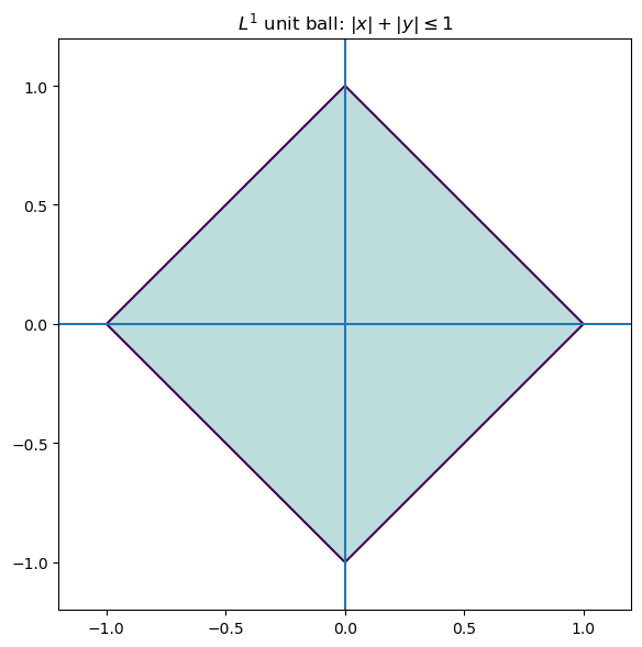
Consequently, optimization problems involving $L^1$ tend to produce solutions which live on the corners of this polytope. Solutions often require linear programming or iterative reweighted least squares.
$L^1$ based methods (such as LASSO) tend to set coefficients to be exactly zero. Unlike with $L^2$, the minimization problem for $L^1$ does not admit a closed-form solution. Algorithms include:
- linear programming formulations,
- iterative reweighted least squares,
- coordinate descent methods.
$L^{\infty}$ norm (max/supremum norm)
The supremum norm defined as $$ |x|_{\infty} = \max |x_i| $$ seeks to control the worst-case error rather than the average error. Minimizing this norm is related to Chebyshev approximation by polynomials.
Geometrically, the unit ball of $\mathbb{R}^2$ with respect to the $L^{\infty}$ norm looks like a square.
import numpy as np
import matplotlib.pyplot as plt

# Grid
xx = np.linspace(-1.2, 1.2, 400)
yy = np.linspace(-1.2, 1.2, 400)
X, Y = np.meshgrid(xx, yy)

# Take the $L^{\infty}$ norm
Z = np.maximum(np.abs(X), np.abs(Y))

plt.figure(figsize=(6,6))
plt.contour(X, Y, Z, levels=[1])
plt.contourf(X, Y, Z, levels=[0,1], alpha=0.3)

plt.axhline(0)
plt.axvline(0)
plt.gca().set_aspect("equal", adjustable="box")
plt.title(r"$L^{\infty}$ unit ball: $\max\{|x|,|y|\} \leq 1$")
plt.tight_layout()
plt.savefig('../images/Linf_unit_ball.png')
plt.show()
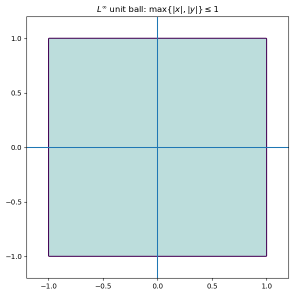
Problems involving the $L^{\infty}$ norm are often formulated as linear programs, and are useful when worst-case guarantees are more important than optimizing average performance.
Matrix norms
There are also various norms on matrices, each highlighting a different aspect of the associated linear transformation.
-
Frobenius norm. This is an important norm, essentially the analogue of the $L^2$ norm for matrices. It is the Euclidean norm if you think of your matrix as a vector, forgetting its rectangular shape. For $A = (a_{ij})$ a matrix, the Frobenius norm $$ |A|F = \sqrt{\sum a{ij}^2} $$ is the square root of the sum of squares of all the entries. This treats a matrix as a long vector and is invariant under orthogonal transformations. As we’ll see, it plays a central role in:
- least-squares problems,
- low-rank approximation,
- principal component analysis.
In particular, the truncated SVD yields a best low-rank approximation of a matrix with respect to the Frobenius norm.
We also note that the Frobenius norm can be written in terms of tracial data. We have that $$ |A|_F^2 = \text{Tr}(A^TA) = \text{Tr}(AA^T). $$
-
Operator norm (spectral norm). This is just the norm as an operator $A: \mathbb{R}^p \to \mathbb{R}^n$, where $\mathbb{R}^p$ and $\mathbb{R}^n$ are thought of as Hilbert spaces: $$ |A| = \max_{|x|_2 = 1}|Ax|_2. $$ This norm measures how big of an amplification $A$ can apply, and is equal to the largest singular value of $A$. This norm is related to stability properties, and is the analogue of the $L^{\infty}$ norm.
-
Nuclear norm. The nuclear norm, defined as $$ |A|_* = \sum \sigma_i, $$ is the sum of the singular values. When $A$ is square, this is precisely the trace-class norm, and is the analogue of the $L^1$ norm. This norm acts as a generalization of the concept of rank.
A note on regularization
Regularization introduces additional constraints or penalties to stabilize ill-posed problems. From the linear algebra point of view, regularization modifies the singular value structure of a problem.
- Ridge regression: add a positive multiple $\lambda\cdot I$ of the identity to $X^TX$ which will artificially inflate small singular values.
- This dampens unstable directions while leaving well-conditioned directions largely unaffected.
Geometrically, regularization reshapes the solution space to suppress directions that are poorly supported by the data.
A note on solving multiple targets concurrently
Suppose now that we were interested in solving several problems concurrently; that is, given some data points, we would like to make $k$ predictions. Say we have our $n \times p$ data matrix $X$, and we want to make $k$ predictions $y_1,\dots,y_k$. We can then set the problem up as finding a best solution to the matrix equation $$ XB = Y $$ where $B$ will be a $p \times k$ matrix of parameters and $Y$ will be the $n \times k$ matrix whose columns are $y_1,\dots,y_k$.
What can go wrong?
We are often dealing with imperfect data, so there is plenty that could go wrong. Here are some basic cases of where things can break down.
-
Perfect multicollinearity: non-invertible $\tilde{X}^T\tilde{X}$. This happens when one feature is a perfect combination of the others. This means that the columns of the matrix $\tilde{X}$ are linearly dependent, and so infinitely many solutions will exist to the least-squares problem.
- For example, if you are looking at characteristics of people and you have height in both inches and centimeters.
-
Almost multicollinearity: this happens when one feature is almost a perfect combination of the others. From the linear algebra perspective, the columns of $\tilde{X}$ might not be dependent, but they will be almost linearly dependent. This will cause problems in calculation, as the condition number will become large and amplify numerical errors. The inverse will blow up small spectral components.
-
More features than observations: this means that our matrix $\tilde{X}$ will be wider than it is high. Necessarily, this means that the columns are linearly dependent. Regularization or dimensionality reduction becomes essential.
-
Redundant or constant features: this is when there is a characteristic that is satisfied by each observation. In terms of the linear algebraic data, this means that one of the columns of $X$ is constant.
- e.g., if you are looking at characteristics of penguins, and you have “# of legs”. This will always be two, and doesn’t add anything to the analysis.
-
Underfitting: the model lacks sufficient expressivity to capture the underlying structure. For example, see the section on polynomial regression – sometimes one might want a curve vs. a straight line.
## Generate data
import numpy as np
import matplotlib.pyplot as plt

# 1) Generate quadratic data
np.random.seed(3)

n = 50
x = np.random.uniform(-5, 5, n)   # symmetric, wider range

# True relationship: y = ax^2 + c + noise
a_true = 2.0
c_true = 5.0
noise = np.random.normal(0, 3, n)

y = a_true * x**2 + c_true + noise

# find a line of best fit
a,b = np.polyfit(x, y, 1)

# add scatter points to plot
plt.scatter(x,y)

# add line of best fit to plot
plt.plot(x, a*x + b, 'r', linewidth=1)

# plot it
plt.show()

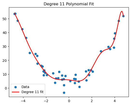
- Overfitting: the model captures noise rather than structure. Often due to model complexity relative to data size. Polynomial regression can give a nice visualization of overfitting. For example, if we worked with the same generated quadratic data from the polynomial regression section, and we tried to approximate it by a degree 11 polynomial, we get the following.
import numpy as np
import matplotlib.pyplot as plt

# 1) Generate quadratic data
np.random.seed(3)

n = 50
x = np.random.uniform(-5, 5, n)

a_true = 2.0
c_true = 5.0
noise = np.random.normal(0, 3, n)

y = a_true * x**2 + c_true + noise

# 2) Fit degree 11 polynomial
coeffs = np.polyfit(x, y, 11)

# Create polynomial function
p = np.poly1d(coeffs)

# 3) Sort x for smooth plotting
x_sorted = np.linspace(min(x), max(x), 500)

# 4) Plot
plt.scatter(x, y, label="Data")
plt.plot(x_sorted, p(x_sorted), 'r', linewidth=2, label="Degree 11 fit")

plt.legend()
plt.title("Degree 11 Polynomial Fit")
plt.show()
-
Outliers: large deviations can dominate the $L^2$ norm. This is where normalization might be key.
-
Heteroscedasticity: this is when the variance of noise changes across observations. Certain least-squares assumptions will break down.
-
Condition number: a large condition number indicates numerical instability and sensitivity to perturbation, even when formal solutions exist.
-
Insufficient tolerance: in numerical algorithms, thresholds used to determine rank or invertibility must be chosen carefully. Poor choices can lead to misleading results.
The point is that many failures in data science are not conceptual; they happen geometrically and numerically. Poor choices lead to poor results.
Principal Component Analysis
Principal Component Analysis (PCA) addresses the issues of multicollinearity and dimensionality mentioned at the end of the previous section by transforming the data into a new coordinate system. The new axes – called principal components – are chosen to capture the maximum variance in the data. In linear algebra terms, we are finding a subspace of potentially smaller dimension that best approximates our data.
Example: Let us return to our house example. Suppose we decide to list the square footage in both square feet and square meters. Let’s add this feature to our dataset.
House Square ft Square m Bedrooms Price (in $1000s) 0 1600 148 3 500 1 2100 195 4 650 2 1550 144 2 475 3 1600 148 3 490 4 2000 185 4 620 In this case, our associated matrix is: $$ X = \begin{bmatrix} 1600 & 148 & 3 & 500 \\ 2100 & 195 & 4 & 650 \\ 1550 & 144 & 2 & 475 \\ 1600 & 148 & 3 & 490 \\ 2000 & 185 & 4 & 620 \end{bmatrix} $$
There are a few problems with the above data and the associated matrix $X$ (this time, we’re not looking to make predictions, so we don’t omit the last column).
- Redundancy: Square feet and square meters give the same information. It’s just a matter of if you’re from a civilized country or from an uncivilized country.
- Numerical instability: The columns of $X$ are nearly linearly dependent. Indeed, the second column is almost a multiple of the first. Moreover, one can make a safe bet that the number of bedrooms increases as the square footage does, so that the first and third columns are correlated.
- Interpretation difficulty: We used the square footage and bedrooms together in the previous section to predict the price of a house. However, because of their correlation, this obfuscates the true relationship, say, between the square footage and the price of a house, or the number of bedrooms and the price of a house.
So the question becomes: what do we do about this? We will try to get a smaller matrix (fewer columns) that contains the same, or a close enough, amount of information. The point is that the data is effectively lower-dimensional.
Let’s do a little analysis on our dataset before progressing. Let’s use pandas.DataFrame.describe, pandas.DataFrame.corr and numpy.linalg.cond. First, let’s set up our data.
import numpy as np
import pandas as pd

# First let us make a dictionary incorporating our data.
# Each entry corresponds to a column (feature of our data)
data = {
    'Square ft': [1600, 2100, 1550, 1600, 2000],
	'Square m': [148, 195, 144, 148, 185],
    'Bedrooms': [3, 4, 2, 3, 4],
    'Price': [500, 650, 475, 490, 620]
}

# Create a pandas DataFrame
df = pd.DataFrame(data)

# Create out matrix X
X = df.to_numpy()
Now let’s see what it has to offer.
df.describe()
| Square ft | Square m | Bedrooms | Price | |
|---|---|---|---|---|
| count | 5.000000 | 5.000000 | 5.00000 | 5.000000 |
| mean | 1770.000000 | 164.000000 | 3.20000 | 547.000000 |
| std | 258.843582 | 24.052027 | 0.83666 | 81.516869 |
| min | 1550.000000 | 144.000000 | 2.00000 | 475.000000 |
| 25% | 1600.000000 | 148.000000 | 3.00000 | 490.000000 |
| 50% | 1600.000000 | 148.000000 | 3.00000 | 500.000000 |
| 75% | 2000.000000 | 185.000000 | 4.00000 | 620.000000 |
| max | 2100.000000 | 195.000000 | 4.00000 | 650.000000 |
df.corr()
| Square ft | Square m | Bedrooms | Price | |
|---|---|---|---|---|
| Square ft | 1.000000 | 0.999886 | 0.900426 | 0.998810 |
| Square m | 0.999886 | 1.000000 | 0.894482 | 0.998395 |
| Bedrooms | 0.900426 | 0.894482 | 1.000000 | 0.909066 |
| Price | 0.998810 | 0.998395 | 0.909066 | 1.000000 |
np.linalg.cond(X)
np.float64(8222.19067218415)
As we can see, everything is basically correlated, and we clearly have some redundancies.
This section is structured as follows.
Low-rank approximation via SVD
Let $A$ be an $n \times p$ matrix and let $A = U\Sigma V^T$ be an SVD. Let $u_1,\dots,u_n$ be the columns of $U$, $v_1,\dots,v_p$ be the columns of $V$, and $\sigma_1 \geq \cdots \geq \sigma_r > 0$ be the singular values, where $r \leq \min{n,p}$ is the rank of $A$. Then we have the reduced singular value decomposition (see Pseudoinverses and using the SVD) $$ A = \sum_{i=1}^r \sigma_i u_iv_i^T $$ (note that $u_i$ is an $n \times 1$ matrix and $v_i$ is a $p \times 1$ matrix, so $u_iv_i^T$ is some $n \times p$ matrix). The key idea is that if the rank of $A$ is higher, say $s$, but the latter singular values are small, then we should still have an approximation like this. Say $\sigma_{r+1},\dots,\sigma_{s}$ are tiny. Then $$ \begin{split} A &= \sum_{i=1}^s \sigma_i u_i v_i^T \\ &= \sum_{i=1}^r \sigma_i u_iv_i^T + \sum_{i=r+1}^{s} \sigma_i u_iv_i^T \\ &\approx \sum_{i=1}^r \sigma_iu_i v_i^T \end{split}. $$ So defining $A_r := \sum_{i=1}^r \sigma_i u_iv_i^T$, we are approximating $A$ by $A_r$.
In what sense is this a good approximation though? Recall that the Frobenius norm of a matrix $A$ is defined as the square root of the sum of the squares of all the entries: $$ |A|F = \sqrt{\sum{i,j} a_{ij}^2}. $$ The Frobenius norm acts as a very nice generalization of the $L^2$ norm for vectors, and is an indispensable tool in both linear algebra and data science. The point is that this “approximation” above actually works in the Frobenius norm, and this reduced singular value decomposition in fact minimizes the error.
Theorem (Eckart–Young–Mirsky). Let $A$ be an $n \times p$ matrix of rank $r$. For $k \leq r$, $$ \min_{B \text{ such that rank}(B) \leq k} |A - B|_F = |A - A_k|_F. $$ The (at most) rank $k$ matrix $A_k$ also realizes the minimum when optimizing for the operator norm.
Example. Recall that we have the following SVD: $$ \begin{bmatrix} 3 & 2 & 2 \\ 2 & 3 & -2 \end{bmatrix} = \begin{bmatrix} \frac{1}{\sqrt{2}} & \frac{1}{\sqrt{2}} \\ \frac{1}{\sqrt{2}} & -\frac{1}{\sqrt{2}} \end{bmatrix} \begin{bmatrix} 5 & 0 & 0 \\ 0 & 3 & 0 \end{bmatrix} \begin{bmatrix} \frac{1}{\sqrt{2}} & \frac{1}{3\sqrt{2}} & -\frac{2}{3} \\ \frac{1}{\sqrt{2}} & -\frac{1}{3\sqrt{2}} & \frac{2}{3} \\ 0 & \frac{4}{3\sqrt{2}} & \frac{1}{3} \end{bmatrix}^T. $$ So if we want a rank-one approximation for the matrix, we’ll do the reduced SVD. We have $$ \begin{split} A_1 &= \sigma_1u_1v_1^T \\ &= 5\begin{bmatrix} \frac{1}{\sqrt{2}} \\ \frac{1}{\sqrt{2}} \end{bmatrix}\begin{bmatrix} \frac{1}{\sqrt{2}} & \frac{1}{\sqrt{2}} & 0 \end{bmatrix} \\ &= \begin{bmatrix} \frac{5}{2} & \frac{5}{2} & 0 \\ \frac{5}{2} & \frac{5}{2} & 0 \end{bmatrix} \end{split}$$ Now let’s compute the (square of the) Frobenius norm of the difference $A - A_1$. We have $$ \begin{split} |A - A_1|_F^2 &= \left| \begin{bmatrix} \frac{1}{2} & -\frac{1}{2} & 2 \\ -\frac{1}{2} & \frac{1}{2} & -2 \end{bmatrix}\right|_F^2 \\ &= 4(\frac{1}{2})^2 + 2(2^2) = 9. \end{split} $$ So the Frobenius distance between $A$ and $A_1$ is 3, and we know by Eckart-Young-Mirsky that this is the smallest we can get when looking at the difference between $A$ and a $2 \times 3$ matrix of rank at most one. As mentioned, the operator norm $|A - A_1|$ also minimizes the distance (in operator norm). We know this to be the largest singular value. As $A - A_1$ has SVD $$ \begin{bmatrix} \frac{1}{2} & -\frac{1}{2} & 2 \\ -\frac{1}{2} & \frac{1}{2} & -2 \end{bmatrix} = \begin{bmatrix} -\frac{1}{\sqrt{2}} & \frac{1}{\sqrt{2}} \\ \frac{1}{\sqrt{2}} & \frac{1}{\sqrt{2}} \end{bmatrix}\begin{bmatrix} 3 & 0 & 0 \\ 0 & 0 & 0 \end{bmatrix} \begin{bmatrix} -\frac{1}{3\sqrt{2}} & -\frac{4}{\sqrt{17}} & \frac{1}{3\sqrt{34}} \\ \frac{1}{3\sqrt{2}} & 0 & \frac{1}{3}\sqrt{\frac{17}{2}} \\ -\frac{2\sqrt{2}}{3} & \frac{1}{\sqrt{17}} & \frac{2}{3}\sqrt{\frac{2}{17}} \end{bmatrix}, $$ the operator norm is also 3.
Now let’s do this in Python. We’ll set up our matrix as usual, take the SVD, do the truncated construction of $A_1$, and use numpy.linalg.norm to look at the norms.
import numpy as np

# Create our matrix A
A = np.array([[3,2,2],[2,3,-2]])

# Take the SVD
U, S, Vh = np.linalg.svd(A)

# Create our rank-1 approximation
sigma1 = S[0]
u1 = U[:, [0]]		#shape (2,2)
v1T = Vh[[0], :]		#shape (3,3)
A1 = sigma1 * (u1 @ v1T)

# Take norms and view errors
frobenius_error = np.linalg.norm(A - A1, ord="fro")	#Frobenius norm
operator_error = np.linalg.norm(A - A1, ord=2)		#operator norm
Let’s see if we get what we expect.
sigma1
np.float64(4.999999999999999)
u1
array([[-0.70710678],
       [-0.70710678]])
v1T
array([[-7.07106781e-01, -7.07106781e-01, -6.47932334e-17]])
A1
array([[2.50000000e+00, 2.50000000e+00, 2.29078674e-16],
       [2.50000000e+00, 2.50000000e+00, 2.29078674e-16]])
frobenius_error
np.float64(3.0)
operator_error
np.float64(3.0)
So this numerically confirms the EYM theorem.
Centering data
In data science, we rarely apply low-rank approximation to raw values directly, because translation and units can dominate the geometry. Instead, we apply these methods to centered (and often standardized) data so that low-rank structure reflects relationships among features rather than the absolute location or measurement scale. Centering converts the problem from approximating an affine cloud to approximating a linear one, in direct analogy with including an intercept term in linear regression. Therefore, before we can analyze the variance structure, we must ensure our data is centered, i.e., that each feature has a mean of 0. We achieve this by subtracting the mean of each column from every entry in that column. Suppose $X$ is our $n \times p$ data matrix, and let $$ \mu = \frac{1}{n}\mathbb{1}^T X. $$ Then $$ \hat{X} = X - \mu \mathbb{1} $$ will be a centered data matrix.
Example. Going back to our housing example, the means of the columns are 1770, 164, 3.2, and 547, respectively. So our centered matrix is $$ \hat{X} = \begin{bmatrix} -170 & -16 & -0.2 & -47 \\ 330 & 31 & 0.8 & 103 \\ -220 & -20 & -1.2 & -72 \\ -170 & -16 & -0.2 & -57 \\ 230 & 21 & 0.8 & 73 \end{bmatrix}. $$
Let’s do this in Python.
import numpy as np
import pandas as pd

# First let us make a dictionary incorporating our data.
# Each entry corresponds to a column (feature of our data)
data = {
    'Square ft': [1600, 2100, 1550, 1600, 2000],
	'Square m': [148, 195, 144, 148, 185],
    'Bedrooms': [3, 4, 2, 3, 4],
    'Price': [500, 650, 475, 490, 620]
}

# Create a pandas DataFrame
df = pd.DataFrame(data)

# Create out matrix X
X = df.to_numpy()

# Get our vector of means
X_means = np.mean(X, axis=0)

# Create our centered matrix
X_centered = X - X_means

# Get the SVD for X_centered
U, S, Vh = np.linalg.svd(X_centered)
This returns the following.
X_means
array([1770. , 164. , 3.2, 547. ])
X_centered
array([[-1.70e+02, -1.60e+01, -2.00e-01, -4.70e+01],
       [ 3.30e+02,  3.10e+01,  8.00e-01,  1.03e+02],
       [-2.20e+02, -2.00e+01, -1.20e+00, -7.20e+01],
       [-1.70e+02, -1.60e+01, -2.00e-01, -5.70e+01],
       [ 2.30e+02,  2.10e+01,  8.00e-01,  7.30e+01]])
We will apply the low-rank approximations from the previous sections. First let’s see what our SVD looks like, and what the condition number is.
print(f"U = {U}\n\nS = {S}\n\nVh.T = {Vh.T}\n")
print("Condition number of X_centered = ", np.linalg.cond(X_centered))
U = [[-0.32486018 -0.81524197 -0.01735449 -0.17188722  0.4472136 ]
 [ 0.63705869  0.10707263 -0.3450375  -0.51345964  0.4472136 ]
 [-0.42643013  0.35553416 -0.61058318  0.34487822  0.4472136 ]
 [-0.33034709  0.436448    0.61781883 -0.3445052   0.4472136 ]
 [ 0.44457871 -0.08381281  0.35515633  0.68497384  0.4472136 ]]

S = [5.44828440e+02 7.61035608e+00 8.91429037e-01 2.41987799e-01]

Vh.T = [[ 0.95017495  0.29361033  0.08182661  0.06530651]
 [ 0.08827897  0.06690917 -0.71081981 -0.69459714]
 [ 0.00276797 -0.04366082  0.69629997 -0.71641638]
 [ 0.29894268 -0.95258064 -0.05662119  0.00417714]]

Condition number of X_centered =  2251.4707027583063
Now let’s approximate our centered matrix $\hat{X}$ by some lower-rank matrices. First, we’ll define a function which will give us a rank $k$ truncated SVD.
# Defining the truncated svd
def reduced_svd_matrix_k(U, S, Vh, k):
	Uk = U[:, :k]
	Sk = np.diag(S[:k])
	Vhk = Vh[:k, :]
	return Uk @ Sk @ Vhk
Now, as $\hat{X}$ has rank 4, we can do a reduced matrix of rank 1,2,3. We will do this in a loop.
Remark. We’ll divide the error by the (Frobenius) norm so that we have a relative error. E.g., if two houses are within 10k of each other, they are similarly priced. The magnitude of error being large doesn’t say much if our quantities are large.
for k in [1, 2, 3]:
	# Define our reduced matrix
    Xck = reduced_svd_matrix_k(U, S, Vh, k)
	# Compute the relative error
    rel_err = np.linalg.norm(X_centered - Xck, ord="fro") / np.linalg.norm(X_centered, ord="fro")
	# Print the information
    print(Xck, "\n", f"k={k}: relative Frobenius reconstruction error on centered data = {rel_err:.4f}", "\n")
[[-168.1743765   -15.62476472   -0.48991109  -52.91078079]
 [ 329.79403078   30.64054254    0.96072753  103.7593243 ]
 [-220.7553464   -20.50996365   -0.64308544  -69.45373002]
 [-171.01485494  -15.88866823   -0.49818573  -53.80444804]
 [ 230.15054706   21.38285405    0.67045472   72.40963456]]
 k=1: relative Frobenius reconstruction error on centered data = 0.0141

[[-1.69996018e+02 -1.60398881e+01 -2.19027093e-01 -4.70007022e+01]
 [ 3.30033282e+02  3.06950642e+01  9.25150039e-01  1.02983104e+02]
 [-2.19960913e+02 -2.03289247e+01 -7.61220318e-01 -7.20311670e+01]
 [-1.70039621e+02 -1.56664278e+01 -6.43206200e-01 -5.69684681e+01]
 [ 2.29963269e+02  2.13401763e+01  6.98303572e-01  7.30172337e+01]]
 k=2: relative Frobenius reconstruction error on centered data = 0.0017

[[-1.69997284e+02 -1.60288915e+01 -2.29799059e-01 -4.69998263e+01]
 [ 3.30008114e+02  3.09136956e+01  7.10984571e-01  1.03000519e+02]
 [-2.20005450e+02 -1.99420315e+01 -1.14021052e+00 -7.20003486e+01]
 [-1.69994556e+02 -1.60579058e+01 -2.59724807e-01 -5.69996518e+01]
 [ 2.29989175e+02  2.11151332e+01  9.18749820e-01  7.29993076e+01]]
 k=3: relative Frobenius reconstruction error on centered data = 0.0004
This seems to check out – it says that rank one (or one feature) should be roughly enough to describe this data. This should make sense because clearly the square meterage, # of bedrooms, and price depend on the square footage.
Mini Project: Image Denoising with the Truncated SVD
This notebook extracts the image denoising project into a standalone workflow and extends it from grayscale images to actual color images.
The core idea is the same as in the original write-up: if an image matrix has singular value decomposition $$ A = U \Sigma V^T, $$ then the best rank-$k$ approximation to $A$ in Frobenius norm is obtained by truncating the SVD. This is the Eckart–Young–Mirsky theorem.
For a grayscale image, the image is a single matrix. For an RGB image, we treat the image as three matrices, one for each channel, and apply truncated SVD to each channel separately.
Outline
- Load an image from disk
- Convert it to grayscale or keep it in RGB
- Add synthetic Gaussian noise
- Compute a truncated SVD reconstruction
- Compare the original, noisy, and denoised images
- Measure quality using MSE and PSNR
This notebook is written so that you can use your own image files directly.
import numpy as np
import matplotlib.pyplot as plt
from PIL import Image
from pathlib import Path

try:
    from skimage.metrics import structural_similarity as ssim
    HAS_SKIMAGE = True
except ImportError:
    ssim = None
    HAS_SKIMAGE = False

print(f"scikit-image available: {HAS_SKIMAGE}")
scikit-image available: True
A note on color images
For a grayscale image, SVD applies directly to a single matrix. For a color image $A \in \mathbb{R}^{n \times p \times 3}$, we write $$ A = (A_R, A_G, A_B), $$ where each channel is an $n \times p$ matrix. We then compute a rank-$k$ approximation for each channel: $$ A_R \approx (A_R)_k,\qquad A_G \approx (A_G)_k,\qquad A_B \approx (A_B)_k, $$ and stack them back together.
This is the most direct extension of the grayscale method, and it works well as a first linear-algebraic treatment of color denoising.
Helper functions
We begin with some utilities for:
- loading images,
- adding Gaussian noise,
- reconstructing rank-$k$ approximations,
- computing image-quality metrics.
def load_image(path, mode="rgb"):
    """
    Load an image from disk.

    Parameters
    ----------
    path : str or Path
        Path to the image file.
    mode : {"rgb", "gray"}
        Whether to load the image as RGB or grayscale.

    Returns
    -------
    np.ndarray
        Float image array scaled to [0, 255].
        Shape is (H, W, 3) for RGB and (H, W) for grayscale.
    """
    path = Path(path)
    if not path.exists():
        raise FileNotFoundError(f"Could not find image file: {path}")

    img = Image.open(path)

    if mode.lower() in {"gray", "grayscale", "l"}:
        img = img.convert("L")
    else:
        img = img.convert("RGB")

    return np.asarray(img, dtype=np.float64)


def show_image(img, title=None):
    """Display a grayscale or RGB image."""
    plt.figure(figsize=(6, 6))
    if img.ndim == 2:
        plt.imshow(np.clip(img, 0, 255), cmap="gray", vmin=0, vmax=255)
    else:
        plt.imshow(np.clip(img, 0, 255).astype(np.uint8))
    if title is not None:
        plt.title(title)
    plt.axis("off")
    plt.tight_layout()
    plt.show()


def add_gaussian_noise(img, sigma=25, seed=0):
    """
    Add Gaussian noise to an image.

    Parameters
    ----------
    img : np.ndarray
        Image array in [0, 255].
    sigma : float
        Standard deviation of the noise.
    seed : int
        Random seed for reproducibility.

    Returns
    -------
    np.ndarray
        Noisy image clipped to [0, 255].
    """
    rng = np.random.default_rng(seed)
    noisy = img + rng.normal(loc=0.0, scale=sigma, size=img.shape)
    return np.clip(noisy, 0, 255)


def truncated_svd_matrix(A, k):
    """
    Return the rank-k truncated SVD approximation of a 2D matrix A.
    """
    U, s, Vt = np.linalg.svd(A, full_matrices=False)
    k = min(k, len(s))
    return (U[:, :k] * s[:k]) @ Vt[:k, :]


def truncated_svd_image(img, k):
    """
    Apply truncated SVD to a grayscale or RGB image.

    For RGB images, truncated SVD is applied channel-by-channel.
    """
    if img.ndim == 2:
        recon = truncated_svd_matrix(img, k)
        return np.clip(recon, 0, 255)

    if img.ndim == 3:
        channels = []
        for c in range(img.shape[2]):
            channel_recon = truncated_svd_matrix(img[:, :, c], k)
            channels.append(channel_recon)
        recon = np.stack(channels, axis=2)
        return np.clip(recon, 0, 255)

    raise ValueError("Image must be either 2D (grayscale) or 3D (RGB).")


def mse(A, B):
    """Mean squared error between two images."""
    return np.mean((A.astype(np.float64) - B.astype(np.float64)) ** 2)


def psnr(A, B, max_val=255.0):
    """Peak signal-to-noise ratio in decibels."""
    err = mse(A, B)
    if err == 0:
        return np.inf
    return 10 * np.log10((max_val ** 2) / err)


def image_ssim(A, B, max_val=255.0):
    """
    Structural similarity index.

    For RGB images, compute SSIM channel-by-channel and average.
    Returns None when scikit-image is unavailable.
    """
    if not HAS_SKIMAGE:
        return None

    A = A.astype(np.float64)
    B = B.astype(np.float64)

    if A.ndim == 2:
        return float(ssim(A, B, data_range=max_val))

    if A.ndim == 3:
        vals = [ssim(A[:, :, c], B[:, :, c], data_range=max_val) for c in range(A.shape[2])]
        return float(np.mean(vals))

    raise ValueError("Images must be either 2D (grayscale) or 3D (RGB).")
Choose an image
from pathlib import Path

MODE = "rgb"  # use "gray" for grayscale, "rgb" for color

candidate_paths = [
    Path("../images/bella.jpg"),
    Path("images/bella.jpg"),
    Path("bella.jpg"),
]

IMAGE_PATH = None
for p in candidate_paths:
    if p.exists():
        IMAGE_PATH = p
        break

if IMAGE_PATH is None:
    raise FileNotFoundError(
        "Could not find bella.jpg. Put it in ../images/, images/, or the notebook folder."
    )

img = load_image(IMAGE_PATH, mode=MODE)
print("Using image:", IMAGE_PATH)
print("Image shape:", img.shape)
show_image(img, title=f"Original image ({MODE})")
Using image: ../images/bella.jpg
Image shape: (3456, 5184, 3)
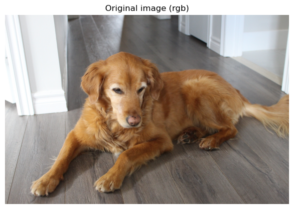
Add synthetic Gaussian noise
We add noise so that the denoising effect is visible and measurable.
sigma = 40
seed = 0

img_noisy = add_gaussian_noise(img, sigma=sigma, seed=seed)

noisy_output_path = IMAGE_PATH.with_name(f"{IMAGE_PATH.stem}_noisy.png")
Image.fromarray(np.clip(img_noisy, 0, 255).astype(np.uint8)).save(noisy_output_path)

show_image(img_noisy, title=f"Noisy image (sigma={sigma})")
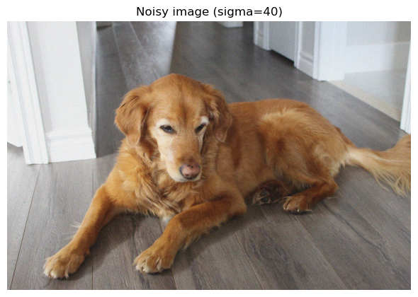
Visualizing rank-$k$ reconstructions
For small $k$, the reconstruction captures only coarse structure. As $k$ increases, more detail returns. For denoising, there is often a useful middle ground: enough singular values to preserve structure, but not so many that we reintroduce noise.
import numpy as np
import matplotlib.pyplot as plt
import math

ks = [5, 20, 50, 100]

# Collect all images + titles
images = []
titles = []

# Original
images.append(img)
titles.append("Original")

# Noisy
images.append(img_noisy)
titles.append("Noisy")

# Reconstructions
for k in ks:
    recon = truncated_svd_image(img_noisy, k)
    images.append(recon)
    titles.append(f"k = {k}")

# Grid setup
ncols = 2
nrows = math.ceil(len(images) / ncols)

fig, axes = plt.subplots(nrows, ncols, figsize=(6 * ncols, 4 * nrows))
axes = axes.flatten()  # easier indexing

# Plot everything
for i, (ax, im, title) in enumerate(zip(axes, images, titles)):
    if im.ndim == 2:
        ax.imshow(im, cmap="gray", vmin=0, vmax=255)
    else:
        ax.imshow(np.clip(im, 0, 255).astype(np.uint8))

    ax.set_title(title)
    ax.axis("off")

# Hide any unused axes
for j in range(len(images), len(axes)):
    axes[j].axis("off")

plt.tight_layout()
comparison_output_path = IMAGE_PATH.with_name(f"{IMAGE_PATH.stem}_truncated_svd_multiple_ks.png")
plt.savefig(comparison_output_path, bbox_inches="tight")
plt.show()
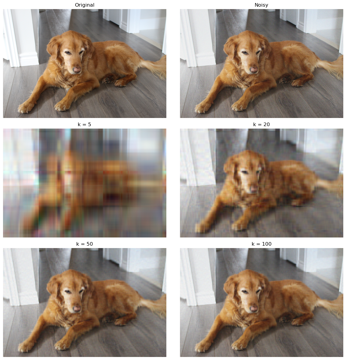
Quantitative evaluation
We compare each reconstruction against the clean original image, not against the noisy one. A good denoising rank should typically:
- reduce MSE relative to the noisy image,
- increase PSNR relative to the noisy image.
baseline_mse = mse(img, img_noisy)
baseline_psnr = psnr(img, img_noisy)

print(f"Noisy image baseline -> MSE: {baseline_mse:.2f}, PSNR: {baseline_psnr:.2f} dB")

results = []
for k in ks:
    recon = truncated_svd_image(img_noisy, k)
    results.append((k, mse(img, recon), psnr(img, recon)))

print("\nRank-k reconstructions:")
for k, m, p in results:
    print(f"k = {k:3d} | MSE = {m:10.2f} | PSNR = {p:6.2f} dB")
Noisy image baseline -> MSE: 1426.31, PSNR: 16.59 dB

Rank-k reconstructions:
k =   5 | MSE =     314.20 | PSNR =  23.16 dB
k =  20 | MSE =     120.90 | PSNR =  27.31 dB
k =  50 | MSE =     104.98 | PSNR =  27.92 dB
k = 100 | MSE =     155.79 | PSNR =  26.21 dB
Efficient search over many values of $k$
A naive implementation would recompute the SVD from scratch for every candidate value of $k$. That is extremely expensive: every reconstruction would require a fresh factorization of each channel of the noisy image.
A much better approach is:
- compute the SVD once for each channel;
- reuse those factors for every candidate $k$;
- compare reconstructions using MSE, PSNR, and optionally SSIM.
This is also a nice numerical linear algebra point: all rank-$k$ truncated reconstructions come from the same singular value decomposition.
We compare two variants:
- plain truncated SVD, applied directly to each channel;
- centered truncated SVD, where we subtract each channel’s column mean before factorizing and add it back after reconstruction.
The centered version sometimes improves reconstruction slightly because the low-rank approximation spends less effort representing the mean structure.
def precompute_svd_image(img):
    """Precompute plain SVD factors for each channel."""
    if img.ndim == 2:
        A = img.astype(np.float64)
        U, s, Vt = np.linalg.svd(A, full_matrices=False)
        return [(U, s, Vt)]

    cache = []
    for c in range(img.shape[2]):
        A = img[:, :, c].astype(np.float64)
        U, s, Vt = np.linalg.svd(A, full_matrices=False)
        cache.append((U, s, Vt))
    return cache


def precompute_centered_svd_image(img):
    """Precompute centered SVD factors for each channel."""
    if img.ndim == 2:
        A = img.astype(np.float64)
        col_mean = A.mean(axis=0, keepdims=True)
        A_centered = A - col_mean
        U, s, Vt = np.linalg.svd(A_centered, full_matrices=False)
        return [(U, s, Vt, col_mean)]

    cache = []
    for c in range(img.shape[2]):
        A = img[:, :, c].astype(np.float64)
        col_mean = A.mean(axis=0, keepdims=True)
        A_centered = A - col_mean
        U, s, Vt = np.linalg.svd(A_centered, full_matrices=False)
        cache.append((U, s, Vt, col_mean))
    return cache


def reconstruct_from_svd_cache(cache, k):
    """Reconstruct from precomputed plain SVD factors."""
    channels = []
    for U, s, Vt in cache:
        kk = min(k, len(s))
        recon = (U[:, :kk] * s[:kk]) @ Vt[:kk, :]
        channels.append(np.clip(recon, 0, 255))

    if len(channels) == 1:
        return channels[0]
    return np.stack(channels, axis=2)


def reconstruct_from_centered_svd_cache(cache, k):
    """Reconstruct from precomputed centered SVD factors."""
    channels = []
    for U, s, Vt, col_mean in cache:
        kk = min(k, len(s))
        recon = (U[:, :kk] * s[:kk]) @ Vt[:kk, :] + col_mean
        channels.append(np.clip(recon, 0, 255))

    if len(channels) == 1:
        return channels[0]
    return np.stack(channels, axis=2)
Scoring reconstructions
We first compute a baseline by comparing the noisy image to the clean one. Then we score
rank-$k$ reconstructions. A smaller MSE and a larger PSNR indicate better fidelity to the clean
image. If scikit-image is available, we also compute SSIM.
A useful conceptual warning is important here:
The best low-rank approximation in a matrix norm does not necessarily produce the image that looks best to a human observer.
Why? Because human perception cares about things like edges, texture, and local contrast, while MSE and PSNR are purely pixelwise. A reconstruction can score well numerically and still look too smooth, too blurry, or otherwise unnatural.
baseline_mse = mse(img, img_noisy)
baseline_psnr = psnr(img, img_noisy)

print(f"Baseline noisy vs clean:")
print(f"  MSE : {baseline_mse:.2f}")
print(f"  PSNR: {baseline_psnr:.2f}")

if HAS_SKIMAGE:
    baseline_ssim = image_ssim(img, img_noisy)
    print(f"  SSIM: {baseline_ssim:.4f}")
Baseline noisy vs clean:
  MSE : 1426.31
  PSNR: 16.59
  SSIM: 0.0674
Automatic search over many values of $k$
Because all rank-$k$ reconstructions come from the same SVD, we precompute the factorizations once and then search efficiently over candidate values of $k$.
For very large images this can still be somewhat expensive, so for exploratory work a coarser grid
such as range(5, 151, 5) is often sufficient. Once a promising region is found, one can refine
the search around that region.
candidate_ks = list(range(1, 151, 5))

plain_cache = precompute_svd_image(img_noisy)
centered_cache = precompute_centered_svd_image(img_noisy)

plain_scores = []
centered_scores = []

for k in candidate_ks:
    plain = reconstruct_from_svd_cache(plain_cache, k)
    centered = reconstruct_from_centered_svd_cache(centered_cache, k)

    plain_row = (k, mse(img, plain), psnr(img, plain))
    centered_row = (k, mse(img, centered), psnr(img, centered))

    if HAS_SKIMAGE:
        plain_row = plain_row + (image_ssim(img, plain),)
        centered_row = centered_row + (image_ssim(img, centered),)

    plain_scores.append(plain_row)
    centered_scores.append(centered_row)

best_plain_by_mse = min(plain_scores, key=lambda x: x[1])
best_plain_by_psnr = max(plain_scores, key=lambda x: x[2])
best_centered_by_mse = min(centered_scores, key=lambda x: x[1])
best_centered_by_psnr = max(centered_scores, key=lambda x: x[2])

print("Plain SVD:")
print("  Best by MSE :", best_plain_by_mse)
print("  Best by PSNR:", best_plain_by_psnr)

print("Centered SVD:")
print("  Best by MSE :", best_centered_by_mse)
print("  Best by PSNR:", best_centered_by_psnr)

if HAS_SKIMAGE:
    best_plain_by_ssim = max(plain_scores, key=lambda x: x[3])
    best_centered_by_ssim = max(centered_scores, key=lambda x: x[3])

    print("Plain SVD:")
    print("  Best by SSIM:", best_plain_by_ssim)
    print("Centered SVD:")
    print("  Best by SSIM:", best_centered_by_ssim)
Plain SVD:
  Best by MSE : (41, np.float64(100.86643831213188), np.float64(28.093336751115086), 0.6093116647651357)
  Best by PSNR: (41, np.float64(100.86643831213188), np.float64(28.093336751115086), 0.6093116647651357)
Centered SVD:
  Best by MSE : (36, np.float64(100.77445519633338), np.float64(28.097299019055427), 0.6300189753895039)
  Best by PSNR: (36, np.float64(100.77445519633338), np.float64(28.097299019055427), 0.6300189753895039)
Plain SVD:
  Best by SSIM: (1, np.float64(1048.5582022585174), np.float64(17.924878190392008), 0.7729763808220854)
Centered SVD:
  Best by SSIM: (1, np.float64(891.0525380576963), np.float64(18.631770492935846), 0.7731825777973053)
Metric curves versus $k$
Plotting the metrics as functions of $k$ is often more informative than looking only at the single best value. Frequently the metric is nearly flat across a whole range of ranks, in which case several nearby values of $k$ have very similar numerical performance.
That is exactly the situation where visual inspection matters most: among a cluster of nearly tied candidates, the one that looks nicest to the eye may not be the exact numerical winner.
plain_ks = [row[0] for row in plain_scores]
plain_mses = [row[1] for row in plain_scores]
plain_psnrs = [row[2] for row in plain_scores]

centered_ks = [row[0] for row in centered_scores]
centered_mses = [row[1] for row in centered_scores]
centered_psnrs = [row[2] for row in centered_scores]

plt.figure(figsize=(8, 4))
plt.plot(plain_ks, plain_mses, label="Plain SVD")
plt.plot(centered_ks, centered_mses, label="Centered SVD")
plt.xlabel("k")
plt.ylabel("MSE")
plt.title("MSE versus rank k")
plt.legend()
plt.tight_layout()
plt.show()

plt.figure(figsize=(8, 4))
plt.plot(plain_ks, plain_psnrs, label="Plain SVD")
plt.plot(centered_ks, centered_psnrs, label="Centered SVD")
plt.xlabel("k")
plt.ylabel("PSNR")
plt.title("PSNR versus rank k")
plt.legend()
plt.tight_layout()
plt.show()

if HAS_SKIMAGE:
    plain_ssims = [row[3] for row in plain_scores]
    centered_ssims = [row[3] for row in centered_scores]

    plt.figure(figsize=(8, 4))
    plt.plot(plain_ks, plain_ssims, label="Plain SVD")
    plt.plot(centered_ks, centered_ssims, label="Centered SVD")
    plt.xlabel("k")
    plt.ylabel("SSIM")
    plt.title("SSIM versus rank k")
    plt.legend()
    plt.tight_layout()
    plt.show()
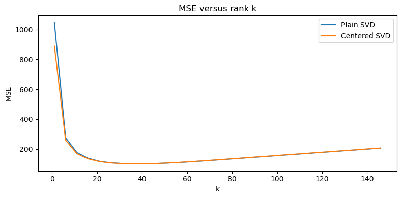
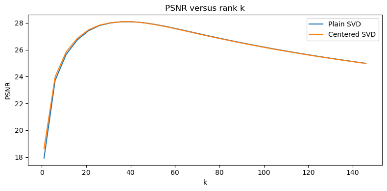
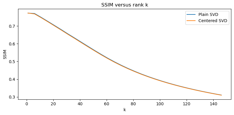
Visual comparison near the best ranks
Finally, we inspect a few reconstructions around the automatically selected ranks. This is important because the reconstruction that is optimal in Frobenius norm, MSE, or PSNR is not guaranteed to be the reconstruction a human would actually prefer.
Low-rank approximation is mathematically optimal for a precise matrix objective, but photographic quality is influenced by far more than that. Fine textures, fur, sharp edges, and local contrast can all matter a great deal perceptually, and some of those are exactly the kinds of features that get smoothed away by aggressive truncation.
# Pick a few candidate ranks around the PSNR-optimal values
plain_best_k = best_plain_by_psnr[0]
centered_best_k = best_centered_by_psnr[0]

plain_inspect_ks = sorted(set(k for k in [plain_best_k - 10, plain_best_k - 5, plain_best_k, plain_best_k + 5, plain_best_k + 10] if k >= 1))
centered_inspect_ks = sorted(set(k for k in [centered_best_k - 10, centered_best_k - 5, centered_best_k, centered_best_k + 5, centered_best_k + 10] if k >= 1))

print("Plain SVD ranks to inspect   :", plain_inspect_ks)
print("Centered SVD ranks to inspect:", centered_inspect_ks)
Plain SVD ranks to inspect   : [31, 36, 41, 46, 51]
Centered SVD ranks to inspect: [26, 31, 36, 41, 46]
import math

# Build a gallery: original, noisy, then several plain and centered reconstructions
gallery_images = [img, img_noisy]
gallery_titles = ["Original", f"Noisy (sigma={sigma})"]

for k in plain_inspect_ks:
    gallery_images.append(reconstruct_from_svd_cache(plain_cache, k))
    gallery_titles.append(f"Plain SVD, k={k}")

for k in centered_inspect_ks:
    gallery_images.append(reconstruct_from_centered_svd_cache(centered_cache, k))
    gallery_titles.append(f"Centered SVD, k={k}")

ncols = 2
nrows = math.ceil(len(gallery_images) / ncols)

fig, axes = plt.subplots(nrows, ncols, figsize=(6 * ncols, 4 * nrows))
axes = np.array(axes).reshape(-1)

for ax, im, title in zip(axes, gallery_images, gallery_titles):
    if im.ndim == 2:
        ax.imshow(im, cmap="gray", vmin=0, vmax=255)
    else:
        ax.imshow(np.clip(im, 0, 255).astype(np.uint8))
    ax.set_title(title)
    ax.axis("off")

for ax in axes[len(gallery_images):]:
    ax.axis("off")

plt.tight_layout()
plt.show()
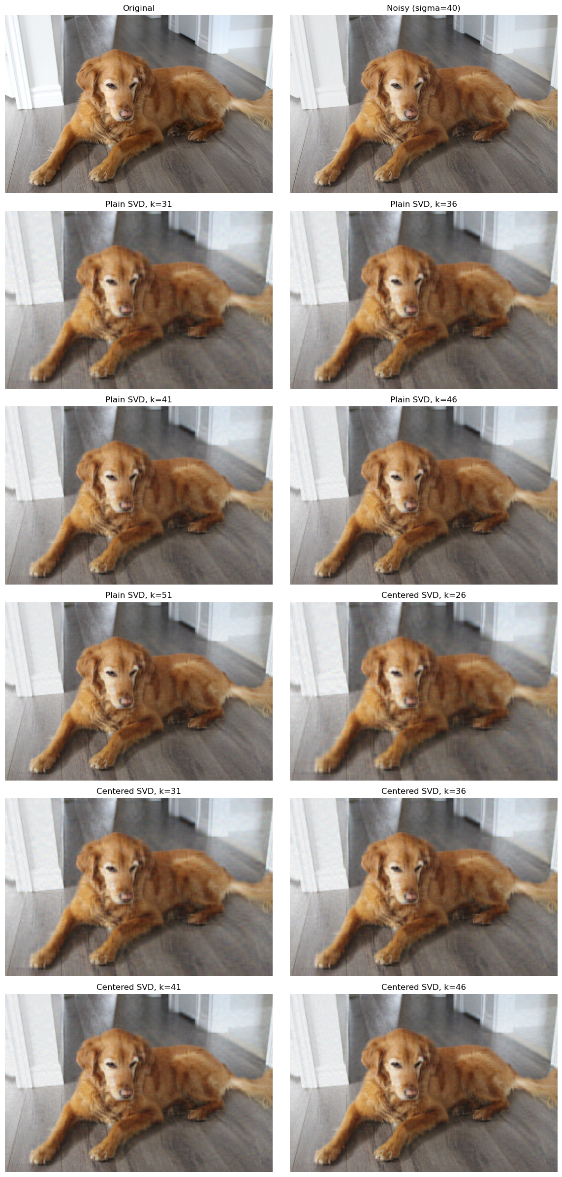
Remarks and possible extensions
- Truncated SVD provides the best rank-$k$ approximation in Frobenius norm, but that does not automatically mean it gives the most visually pleasing denoised image.
- For real photographs, low-rank methods often smooth away texture and local detail along with the noise.
- The visually best image may lie near the metric optimum rather than exactly at it.
- One can compare this method with more perceptual denoisers such as wavelet methods, bilateral filtering, non-local means, or modern learned denoisers.
- A useful next step would be to compare how the preferred $k$ changes as the noise level $\sigma$ increases.
Modelling 101: Train/Test Splits & Beyond Linear Regression
Introduction
So far we have seen how linear regression (ordinary least squares) solves $\tilde{X}\tilde{\beta} = y$ by minimizing $|y - \tilde{X}\tilde{\beta}|_2^2$. This is a powerful tool, but real data often breaks the assumptions that make linear regression the best choice. We address several of the points made in notebook 03.
Why linear regression might not cut it:
- Nonlinear relationships – The true dependency may be curved, periodic, or otherwise not linear.
- High dimensionality – When the number of features $p$ is close to or larger than the number of observations $n$, the matrix $\tilde{X}^T\tilde{X}$ becomes singular or nearly singular.
- Multicollinearity – Features are correlated, leading to large condition numbers and unstable coefficients.
- Overfitting – A complex model fits noise instead of signal, especially when $p$ is large.
- Outliers – The $L^2$ norm magnifies large errors, pulling the fit away from the bulk of the data.
In this notebook we will:
- Work with a real, moderately sized dataset.
- Learn how to properly split data into training, validation, and test sets.
- Apply linear and polynomial regression, then diagnose their limitations.
- Introduce regularisation methods (Ridge and Lasso) from a linear algebra perspective.
- Explore gradient descent as a numerical optimisation alternative to the normal equations.
- Look at decision trees and random forests – nonlinear models that can capture complex interactions without feature engineering.
- Cover logistic regression for classification.
- Discuss feature scaling, cross‑validation, model interpretation, and hyperparameter tuning.
The goal is to equip the linear algebraist with practical modelling tools while maintaining a geometric/algebraic intuition.
A Real Dataset: California Housing
A natural next step from our toy housing example is the California housing dataset from sklearn.datasets. It contains 20,640 observations of 8 features (median income, house age, average rooms, etc.) and the target is the median house value for blocks in California. This dataset is large enough to illustrate interesting effects but small enough to run quickly.
Linear algebra view: Each observation is a row vector $x_i \in \mathbb{R}^8$. The features form the columns of the design matrix $X \in \mathbb{R}^{20640 \times 8}$. We will add an intercept column $\mathbb{1}$ to obtain $\tilde{X} \in \mathbb{R}^{20640 \times 9}$.
import numpy as np
import pandas as pd
import matplotlib.pyplot as plt
from sklearn.datasets import fetch_california_housing

# Load the data
housing = fetch_california_housing()
X = housing.data          # shape (20640, 8)
y = housing.target       # shape (20640,)
feature_names = housing.feature_names

# Convert to DataFrame for convenience
df = pd.DataFrame(X, columns=feature_names)
df['MedHouseVal'] = y

print(f"Data shape: {df.shape}")
df.head()
Data shape: (20640, 9)
| MedInc | HouseAge | AveRooms | AveBedrms | Population | AveOccup | Latitude | Longitude | MedHouseVal | |
|---|---|---|---|---|---|---|---|---|---|
| 0 | 8.3252 | 41.0 | 6.984127 | 1.023810 | 322.0 | 2.555556 | 37.88 | -122.23 | 4.526 |
| 1 | 8.3014 | 21.0 | 6.238137 | 0.971880 | 2401.0 | 2.109842 | 37.86 | -122.22 | 3.585 |
| 2 | 7.2574 | 52.0 | 8.288136 | 1.073446 | 496.0 | 2.802260 | 37.85 | -122.24 | 3.521 |
| 3 | 5.6431 | 52.0 | 5.817352 | 1.073059 | 558.0 | 2.547945 | 37.85 | -122.25 | 3.413 |
| 4 | 3.8462 | 52.0 | 6.281853 | 1.081081 | 565.0 | 2.181467 | 37.85 | -122.25 | 3.422 |
# Basic statistics
df.describe()
| MedInc | HouseAge | AveRooms | AveBedrms | Population | AveOccup | Latitude | Longitude | MedHouseVal | |
|---|---|---|---|---|---|---|---|---|---|
| count | 20640.000000 | 20640.000000 | 20640.000000 | 20640.000000 | 20640.000000 | 20640.000000 | 20640.000000 | 20640.000000 | 20640.000000 |
| mean | 3.870671 | 28.639486 | 5.429000 | 1.096675 | 1425.476744 | 3.070655 | 35.631861 | -119.569704 | 2.068558 |
| std | 1.899822 | 12.585558 | 2.474173 | 0.473911 | 1132.462122 | 10.386050 | 2.135952 | 2.003532 | 1.153956 |
| min | 0.499900 | 1.000000 | 0.846154 | 0.333333 | 3.000000 | 0.692308 | 32.540000 | -124.350000 | 0.149990 |
| 25% | 2.563400 | 18.000000 | 4.440716 | 1.006079 | 787.000000 | 2.429741 | 33.930000 | -121.800000 | 1.196000 |
| 50% | 3.534800 | 29.000000 | 5.229129 | 1.048780 | 1166.000000 | 2.818116 | 34.260000 | -118.490000 | 1.797000 |
| 75% | 4.743250 | 37.000000 | 6.052381 | 1.099526 | 1725.000000 | 3.282261 | 37.710000 | -118.010000 | 2.647250 |
| max | 15.000100 | 52.000000 | 141.909091 | 34.066667 | 35682.000000 | 1243.333333 | 41.950000 | -114.310000 | 5.000010 |
Let’s see the relationships between these features and the price.
Train / Test Split (and Validation)
When it comes to real-world modelling, we must split our data into training and test sets.
Why split? If we evaluate a model on the same data we used to train it, we get an overly optimistic estimate of performance. The model may have memorised the training set (overfitting). Splitting mimics a real‑world scenario: we test on unseen data.
A common workflow:
- Training set (e.g., 60‑80%): used to fit the model parameters.
- Validation set (e.g., 10‑20%): used to tune hyperparameters (e.g., degree of polynomial, regularisation strength).
- Test set (e.g., 10‑20%): used only once at the end to report final performance.
# Illustrate the three-way split
fig, ax = plt.subplots(figsize=(12, 3))

# Create rectangles for each split
ax.barh(0, 60, left=0, height=0.5, color='blue', alpha=0.7, label='Training (60%)')
ax.barh(0, 20, left=60, height=0.5, color='orange', alpha=0.7, label='Validation (20%)')
ax.barh(0, 20, left=80, height=0.5, color='red', alpha=0.7, label='Test (20%)')

# Add labels
ax.text(30, 0, 'Train Model\nParameters', ha='center', va='center', fontsize=10, fontweight='bold')
ax.text(70, 0, 'Tune\nHyperparams', ha='center', va='center', fontsize=10, fontweight='bold')
ax.text(90, 0, 'Final\nEvaluation', ha='center', va='center', fontsize=10, fontweight='bold')

ax.set_xlim(0, 100)
ax.set_ylim(-0.5, 0.5)
ax.set_xlabel('Percentage of Data')
ax.set_yticks([])
ax.set_title('Train/Validation/Test Split')
ax.legend(loc='upper center', bbox_to_anchor=(0.5, -0.15), ncol=3)

plt.tight_layout()
plt.savefig('../images/train_validation_test_split.png')
plt.show()
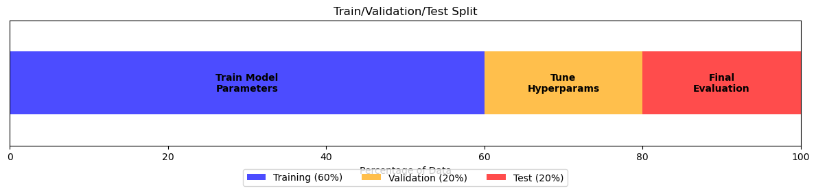
Let us first fix a random state.
RANDOM_STATE=3
Let’s visualize this.
import numpy as np
import matplotlib.pyplot as plt
from sklearn.model_selection import train_test_split

# Generate synthetic data to illustrate the concept
np.random.seed(3)
n = 50
X = np.random.uniform(-5,5,n) # synthetic, wider range

# True relationship
a_true = 2.0
c_true = 5.0
noise = np.random.normal(0,3,n)

y = a_true * X**2 + c_true + noise

# Perform train/test split
X_train, X_test, y_train, y_test = train_test_split(
    X,y, test_size=0.3, random_state=3
)

# Sort for plotting
X_curve = np.linspace(X.min(), X. max())
y_true = a_true * X_curve**2 + c_true


# Plot
fig, ax = plt.subplots(figsize=(10,6))
ax.scatter(X_train, y_train, color='blue', s=50, label='Training data', zorder=3)
ax.scatter(X_test, y_test, color='red', s=50, label='Test data', zorder=3)
ax.plot(X_curve, y_true, linewidth=2, label='True relationship', alpha=0.7)

ax.set_xlabel('X')
ax.set_ylabel('y')
ax.set_title('Train/Test Split')
ax.legend()
ax.grid(True, alpha=0.3)
plt.tight_layout()
plt.savefig('../images/train_test_split_illustration.png')
plt.show()

print(f"Total samples: {n}")
print(f"Training samples: {len(X_train)} ({len(X_train)/n*100:.0f}%)")
print(f"Test samples: {len(X_test)} ({len(X_test)/n*100:.0f}%)")
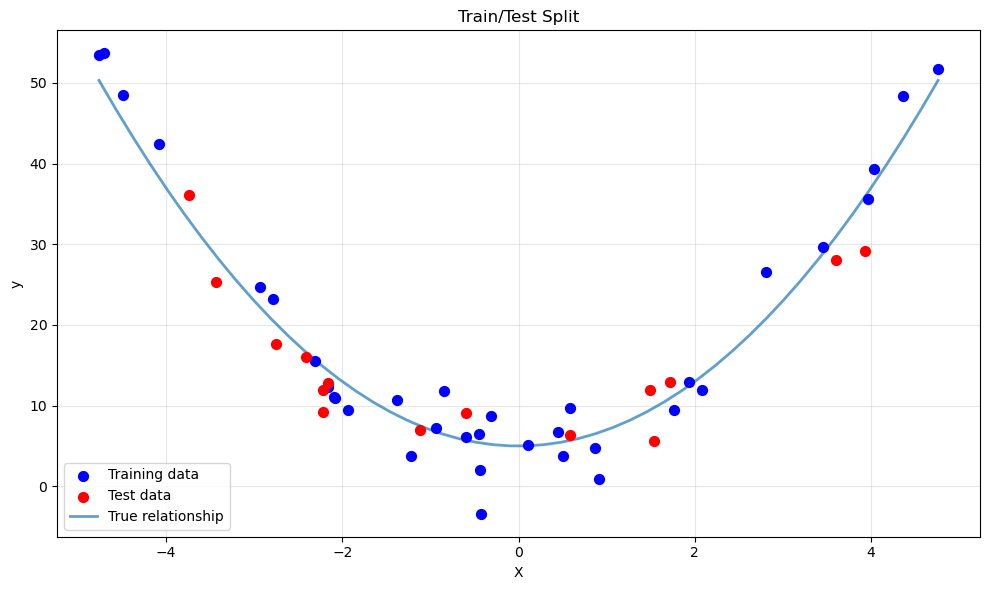
Total samples: 50
Training samples: 35 (70%)
Test samples: 15 (30%)
Back to the housing data. We will use sklearn.model_selection.train_test_split to create two splits (train+validation vs. test), then further split the train+validation part if needed. For simplicity we will first do a single train/test split and use cross‑validation later.
from sklearn.model_selection import train_test_split

# Separate features and target
X = df[feature_names].values
y = df['MedHouseVal'].values

# Split: 80% train, 20% test
X_train, X_test, y_train, y_test = train_test_split(X, y, test_size=0.2, random_state=RANDOM_STATE)

print(f"Training set size: {X_train.shape[0]}")
print(f"Test set size:     {X_test.shape[0]}")
Training set size: 16512
Test set size:     4128
With that, let’s see the relationship between the features and the price.
# Visualize relationships between features and target
fig, axes = plt.subplots(2, 4, figsize=(16, 8))
axes = axes.flatten()

for i, (name, ax) in enumerate(zip(feature_names, axes)):
    ax.scatter(X_train[:, i], y_train, alpha=0.1, s=1)
    ax.set_xlabel(name)
    ax.set_ylabel('MedHouseVal')
    ax.set_title(f'{name} vs Price')

plt.tight_layout()
plt.savefig('../images/california_housing_scatter.png')
plt.show()
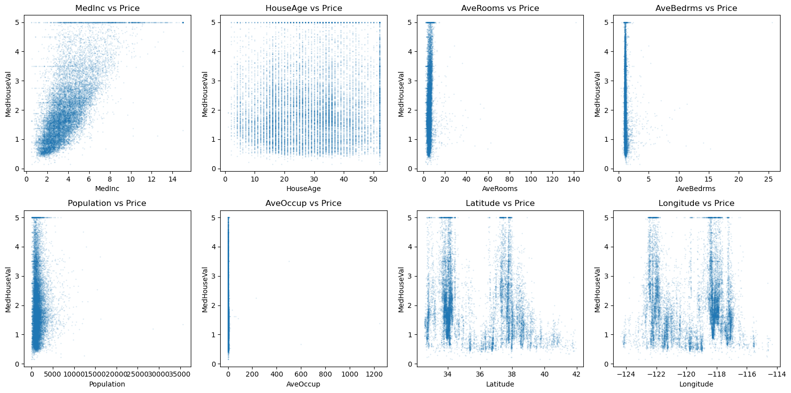
Linear Regression in Practice
We can use sklearn.linear_model.LinearRegression, which internally solves the normal equations using either a direct solver or an SVD‑based approach (the lstsq method we saw earlier).
Linear algebra reminder: The least‑squares solution minimises $|y - X\beta|_2^2$. The closed form is $\beta = (X^T X)^{-1} X^T y$ when $X$ has full column rank.
from sklearn.linear_model import LinearRegression
from sklearn.metrics import mean_squared_error, r2_score

# Fit linear regression
lin_reg = LinearRegression()
lin_reg.fit(X_train, y_train)

# Predict on train and test
y_train_pred = lin_reg.predict(X_train)
y_test_pred = lin_reg.predict(X_test)

# Evaluate
train_mse = mean_squared_error(y_train, y_train_pred)
test_mse = mean_squared_error(y_test, y_test_pred)
train_r2 = r2_score(y_train, y_train_pred)
test_r2 = r2_score(y_test, y_test_pred)

print(f"Train MSE: {train_mse:.4f},  Train R²: {train_r2:.4f}")
print(f"Test  MSE: {test_mse:.4f},  Test  R²: {test_r2:.4f}")
Train MSE: 0.5229,  Train R²: 0.6079
Test  MSE: 0.5381,  Test  R²: 0.5931
The test $R^2$ is respectable (~0.6), but perhaps we can do better with a more flexible model. However, simply adding polynomial features might lead to overfitting. Let’s examine that.
Polynomial Regression and the Danger of Overfitting
Polynomial regression creates new features by taking powers of the original features. For example, with one feature $x$, a degree‑2 model uses $[1, x, x^2]$. For multiple features, we can include interaction terms.
Linear algebra view: The Vandermonde matrix (for one feature) or its multivariate generalisation becomes the new design matrix. As degree increases, the condition number often explodes, leading to numerical instability and wild coefficients – a sign of overfitting.
Let’s illustrate underfitting and overfitting on synthetic data before moving to the housing dataset.
Illustration: Underfitting vs Overfitting
We generate data from a quadratic function with noise, then fit polynomials of different degrees.
# Generate quadratic data (similar to notebook 02) – using distinct names
np.random.seed(3)
n_synth = 50
x_synth = np.random.uniform(-5, 5, n_synth)
y_true_synth = 2.0 * x_synth**2 + 5.0
noise_synth = np.random.normal(0, 3, n_synth)
y_synth = y_true_synth + noise_synth

# Fit polynomials of degree 1 (underfit), 2 (good), 11 (overfit)
degrees = [1, 2, 11]
x_plot = np.linspace(-5, 5, 200)

fig, axes = plt.subplots(1, 3, figsize=(15, 4))
for idx, d in enumerate(degrees):
    coeff = np.polyfit(x_synth, y_synth, d)
    p = np.poly1d(coeff)
    axes[idx].scatter(x_synth, y_synth, alpha=0.7, label='Data')
    axes[idx].plot(x_plot, p(x_plot), 'r-', linewidth=2, label=f'Degree {d}')
    axes[idx].set_title(f'Degree {d} fit')
    axes[idx].set_xlabel('x')
    axes[idx].set_ylabel('y')
    axes[idx].legend()
    axes[idx].grid(True)
plt.tight_layout()
plt.savefig('../images/underfitting_vs_overfitting.png')
plt.show()
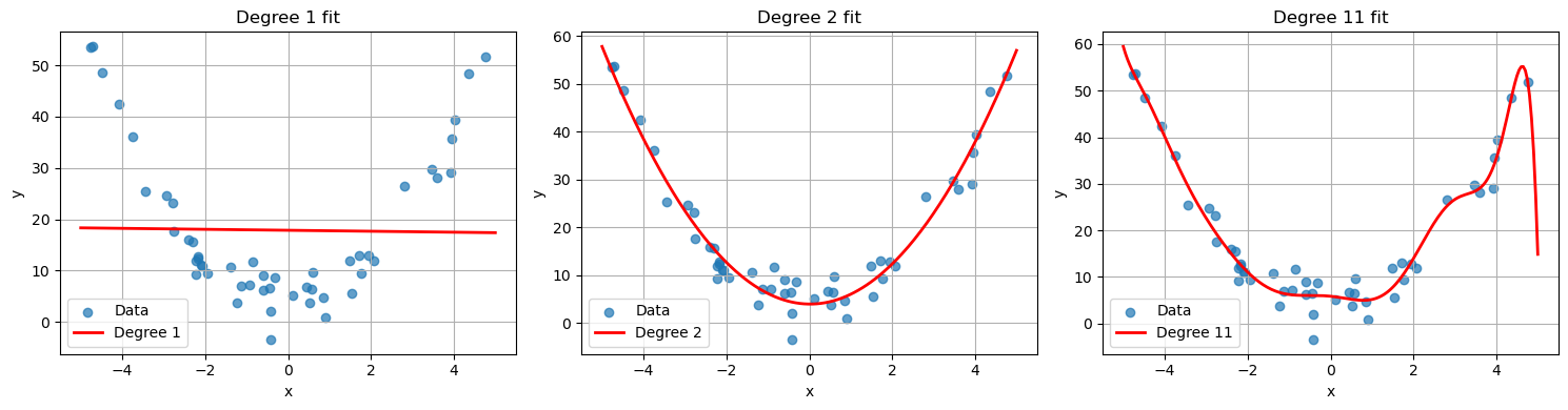
- Degree 1 (underfitting): The linear model cannot capture the curvature, resulting in high bias.
- Degree 2 (good): The quadratic model matches the true underlying structure.
- Degree 11 (overfitting): The polynomial oscillates wildly to fit the noise, leading to poor generalisation.
Now back to the housing dataset. Let’s create polynomial features and see the effect on condition number and test error.
from sklearn.preprocessing import PolynomialFeatures

# Create polynomial features of degree 2 (includes interactions)
poly = PolynomialFeatures(degree=2, include_bias=False)
X_train_poly = poly.fit_transform(X_train)
X_test_poly = poly.transform(X_test)

print(f"Original training features: {X_train.shape[1]}")
print(f"Polynomial training features: {X_train_poly.shape[1]}")

# Condition number of the augmented polynomial design matrix (with intercept added later)
from numpy.linalg import cond

X_train_poly_with_intercept = np.hstack([np.ones((X_train_poly.shape[0], 1)), X_train_poly])
print(f"Condition number of polynomial design matrix: {cond(X_train_poly_with_intercept):.2e}")
Original training features: 8
Polynomial training features: 44
Condition number of polynomial design matrix: 1.55e+11
# Fit linear regression on polynomial features
poly_reg = LinearRegression()
poly_reg.fit(X_train_poly, y_train)

y_train_pred_poly = poly_reg.predict(X_train_poly)
y_test_pred_poly = poly_reg.predict(X_test_poly)

train_mse_poly = mean_squared_error(y_train, y_train_pred_poly)
test_mse_poly = mean_squared_error(y_test, y_test_pred_poly)

print(f"Polynomial (deg=2) Train MSE: {train_mse_poly:.4f}")
print(f"Polynomial (deg=2) Test  MSE: {test_mse_poly:.4f}")
Polynomial (deg=2) Train MSE: 0.4217
Polynomial (deg=2) Test  MSE: 0.4669
The test error is worse than the linear model – this is a clear sign of overfitting. The model is too flexible and fits noise in the training data. We need regularisation.
Ridge Regression ($L^2$ Regularisation)
Ridge regression adds a penalty on the squared $L^2$ norm of the coefficient vector:
$$ \min_{\beta} |y - X\beta|_2^2 + \lambda |\beta|_2^2 $$
where $\lambda \ge 0$ is the regularisation strength.
Linear algebra interpretation: The normal equations become $(X^T X + \lambda I)\beta = X^T y$. Adding $\lambda I$ to $X^T X$ increases all eigenvalues by $\lambda$, thereby improving the condition number and making the problem well‑posed even when $X^T X$ is singular. This is a form of Tikhonov regularisation. This directly shifts the eigenvalues (and singular values) of $X^TX$.
Ridge regression shrinks coefficients towards zero but rarely makes them exactly zero. It is especially useful when features are correlated (multicollinearity).
from sklearn.linear_model import Ridge
from sklearn.model_selection import cross_val_score

# We'll use the polynomial features because ridge can help with overfitting
# Choose lambda via cross-validation on the training set
alphas = np.logspace(-3, 3, 20)
cv_scores = []

for alpha in alphas:
    ridge = Ridge(alpha=alpha)
    # 5-fold cross-validation, negative MSE (scoring expects higher = better)
    scores = cross_val_score(ridge, X_train_poly, y_train, cv=5, scoring='neg_mean_squared_error')
    cv_scores.append(-scores.mean())

best_alpha = alphas[np.argmin(cv_scores)]
print(f"Best alpha from CV: {best_alpha:.4f}")

# Plot CV error vs alpha
plt.figure(figsize=(8,4))
plt.semilogx(alphas, cv_scores)
plt.xlabel('alpha (λ)')
plt.ylabel('Cross-validated MSE')
plt.title('Ridge Regularisation on Polynomial Features')
plt.grid(True)
plt.savefig('../images/ridge_regularization_polynomial_features_unscaled.png')
plt.show()
/usr/lib64/python3.14/site-packages/scipy/_lib/_util.py:1233: LinAlgWarning: Ill-conditioned matrix (rcond=5.61091e-21): result may not be accurate.
  return f(*arrays, *other_args, **kwargs)
/usr/lib64/python3.14/site-packages/scipy/_lib/_util.py:1233: LinAlgWarning: Ill-conditioned matrix (rcond=1.8355e-20): result may not be accurate.
  return f(*arrays, *other_args, **kwargs)
/usr/lib64/python3.14/site-packages/scipy/_lib/_util.py:1233: LinAlgWarning: Ill-conditioned matrix (rcond=6.12863e-21): result may not be accurate.
  return f(*arrays, *other_args, **kwargs)
/usr/lib64/python3.14/site-packages/scipy/_lib/_util.py:1233: LinAlgWarning: Ill-conditioned matrix (rcond=6.2106e-21): result may not be accurate.
...


Best alpha from CV: 1000.0000
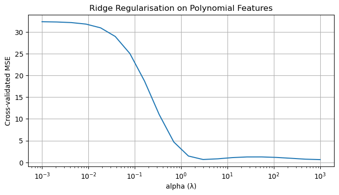
You’ll notice we are getting a bunch of warnings about ill-conditioned matrices. This happens because the polynomial features are on wildly different scales. Let’s standardize our features first.
from sklearn.linear_model import Ridge
from sklearn.model_selection import cross_val_score
from sklearn.preprocessing import StandardScaler

# Add scaler
scaler = StandardScaler()
X_train_poly_scaled = scaler.fit_transform(X_train_poly)
X_test_poly_scaled = scaler.transform(X_test_poly)

# We'll use the polynomial features because ridge can help with overfitting
# Choose lambda via cross-validation on the training set
alphas = np.logspace(-3, 3, 20)
cv_scores = []

for alpha in alphas:
    ridge = Ridge(alpha=alpha)
    scores = cross_val_score(ridge, X_train_poly_scaled, y_train, cv=5, scoring='neg_mean_squared_error')
    cv_scores.append(-scores.mean())

best_alpha = alphas[np.argmin(cv_scores)]
print(f"Best alpha from CV: {best_alpha:.4f}")

# Plot CV error vs alpha
plt.figure(figsize=(8,4))
plt.semilogx(alphas, cv_scores)
plt.xlabel('alpha (λ)')
plt.ylabel('Cross-validated MSE')
plt.title('Ridge Regularisation on Polynomial Features')
plt.grid(True)
plt.savefig('../images/ridge_regularization_polynomial_features_scaled.png')
plt.show()
Best alpha from CV: 233.5721
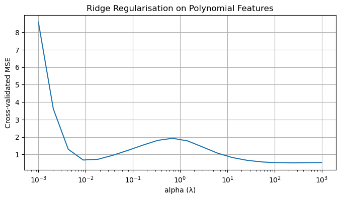
# Fit ridge with best alpha on SCALED polynomial features
ridge_best = Ridge(alpha=best_alpha)
ridge_best.fit(X_train_poly_scaled, y_train)

y_test_pred_ridge = ridge_best.predict(X_test_poly_scaled)
test_mse_ridge = mean_squared_error(y_test, y_test_pred_ridge)
print(f"Ridge (poly deg=2) Test MSE: {test_mse_ridge:.4f}")
print(f"Ridge vs. plain polynomial (MSE {test_mse_poly:.4f} -> {test_mse_ridge:.4f})")
Ridge (poly deg=2) Test MSE: 0.4791
Ridge vs. plain polynomial (MSE 0.4669 -> 0.4791)
Ridge from the SVD Perspective
The Ridge solution has a beautiful interpretation in terms of singular values. Recall from Notebook 2 that if $X = U\Sigma V^T$ is the SVD of the (centered) design matrix, then the OLS solution is
$$ \tilde{\beta}_{OLS} = V\Sigma^{-1}U^T y = \sum_{i=1}^{p} \frac{1}{\sigma_i} (u_i^T y) v_i. $$
When $\sigma_i$ is small, the coefficient $\frac{1}{\sigma_i}$ explodes — this is the condition number problem.
For Ridge regression, one can show that
$$ \tilde{\beta}_{Ridge} = \sum_{i=1}^{p} \frac{\sigma_i}{\sigma_i^2 + \lambda} (u_i^T y) v_i. $$
Notice what happens:
- When $\sigma_i \gg \sqrt{\lambda}$, the coefficient is approximately $\frac{1}{\sigma_i}$ (same as OLS).
- When $\sigma_i \ll \sqrt{\lambda}$, the coefficient is approximately $\frac{\sigma_i}{\lambda}$ — shrunk towards zero.
- The effective condition number becomes $\frac{\sigma_1^2 + \lambda}{\sigma_p^2 + \lambda}$, which is much better than $\frac{\sigma_1^2}{\sigma_p^2}$.
This is why Ridge helps with multicollinearity: it dampens precisely those directions that were poorly determined.
# Visualize how Ridge shrinks coefficients relative to singular values
from sklearn.preprocessing import StandardScaler

# Use scaled data for clean SVD interpretation
scaler = StandardScaler()
X_train_scaled = scaler.fit_transform(X_train)

# Compute SVD of centered design matrix
U, s, Vt = np.linalg.svd(X_train_scaled, full_matrices=False)

# For different lambda values, compute the "shrinkage factor" for each singular direction
lambdas = [0, 0.1, 1, 10, 100]

plt.figure(figsize=(10, 5))

for lam in lambdas:
    if lam == 0:
        # OLS: no shrinkage
        shrinkage = np.ones_like(s)
        label = 'OLS (λ=0)'
    else:
        # Ridge shrinkage factor: sigma / (sigma^2 + lambda)
        shrinkage = s / (s**2 + lam)
        # Normalize so we can compare shapes
        shrinkage = shrinkage / shrinkage[0]  # normalize to first component
        label = f'Ridge (λ={lam})'

    plt.plot(range(1, len(s)+1), shrinkage, 'o-', label=label, markersize=8)

plt.xlabel('Singular value index (decreasing)')
plt.ylabel('Shrinkage factor (normalized)')
plt.title('Ridge Shrinkage: How λ Dampens Small Singular Directions')
plt.legend()
plt.grid(True, alpha=0.3)
plt.xticks(range(1, len(s)+1))
plt.tight_layout()
plt.savefig('../images/ridge_svd_shrinkage.png')
plt.show()

# Show condition number improvement
print("Singular values:", s.round(2))
print(f"\nCondition number (OLS): {s[0]/s[-1]:.2f}")
for lam in [0.1, 1, 10]:
    effective_cond = (s[0]**2 + lam) / (s[-1]**2 + lam)
    print(f"Effective condition number (λ={lam}): {effective_cond:.2f}")
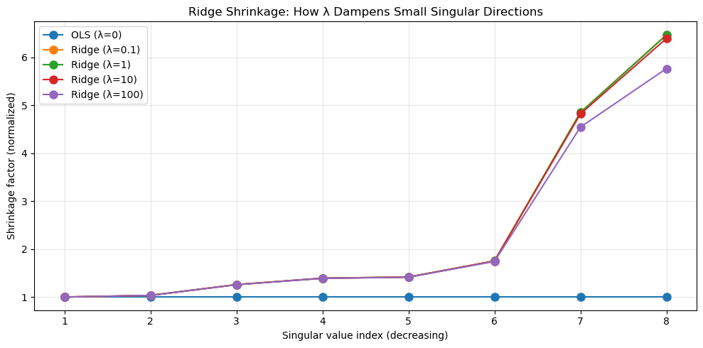
Singular values: [182.41 176.4  144.85 130.91 128.68 104.03  37.56  28.16]

Condition number (OLS): 6.48
Effective condition number (λ=0.1): 41.96
Effective condition number (λ=1): 41.91
Effective condition number (λ=10): 41.45
Lasso Regression ($L^1$ Regularisation)
Lasso replaces the $L^2$ penalty with an $L^1$ penalty:
$$ \min_{\beta} |y - X\beta|_2^2 + \lambda |\beta|_1 $$
Geometric intuition: The $L^1$ ball is a diamond (in $\mathbb{R}^2$). The intersection of the quadratic loss contours with this diamond often occurs at a corner, forcing some coefficients to be exactly zero. Thus Lasso performs feature selection.
Lasso is useful when we suspect that only a few features are truly relevant, especially in high‑dimensional settings. However, it does not have a closed‑form solution; it is typically solved via coordinate descent or other optimisation algorithms.
from sklearn.linear_model import Lasso

# Lasso also requires tuning of alpha
lasso = Lasso(alpha=0.01, max_iter=10000)  # start with a small alpha
lasso.fit(X_train_poly, y_train)

# Count non-zero coefficients
n_nonzero = np.sum(np.abs(lasso.coef_) > 1e-10)
print(f"Number of non-zero coefficients: {n_nonzero} out of {len(lasso.coef_)}")

y_test_pred_lasso = lasso.predict(X_test_poly)
test_mse_lasso = mean_squared_error(y_test, y_test_pred_lasso)
print(f"Lasso (poly deg=2) Test MSE: {test_mse_lasso:.4f}")

# Cross-validation for Lasso alpha
from sklearn.linear_model import LassoCV

lasso_cv = LassoCV(alphas=np.logspace(-3, 1, 30), cv=5, max_iter=10000, random_state=RANDOM_STATE)
lasso_cv.fit(X_train_poly, y_train)
print(f"Best alpha from LassoCV: {lasso_cv.alpha_:.4f}")
print(f"Number of non-zero coefficients (CV best): {np.sum(np.abs(lasso_cv.coef_) > 1e-10)}")

y_test_pred_lasso_cv = lasso_cv.predict(X_test_poly)
test_mse_lasso_cv = mean_squared_error(y_test, y_test_pred_lasso_cv)
print(f"LassoCV Test MSE: {test_mse_lasso_cv:.4f}")
/home/$USER/.local/lib/python3.14/site-packages/sklearn/linear_model/_coordinate_descent.py:716: ConvergenceWarning: Objective did not converge. You might want to increase the number of iterations, check the scale of the features or consider increasing regularisation. Duality gap: 3.725e+03, tolerance: 2.202e+00
  model = cd_fast.enet_coordinate_descent(


Number of non-zero coefficients: 33 out of 44
Lasso (poly deg=2) Test MSE: 0.4538


/home/$USER/.local/lib/python3.14/site-packages/sklearn/linear_model/_coordinate_descent.py:701: ConvergenceWarning: Objective did not converge. You might want to increase the number of iterations, check the scale of the features or consider increasing regularisation. Duality gap: 2.501e+03, tolerance: 1.774e+00
  model = cd_fast.enet_coordinate_descent_gram(
/home/$USER/.local/lib/python3.14/site-packages/sklearn/linear_model/_coordinate_descent.py:701: ConvergenceWarning: Objective did not converge. You might want to increase the number of iterations, check the scale of the features or consider increasing regularisation. Duality gap: 3.286e+03, tolerance: 1.774e+00
  model = cd_fast.enet_coordinate_descent_gram(
/home/$USER/.local/lib/python3.14/site-packages/sklearn/linear_model/_coordinate_descent.py:701: ConvergenceWarning: Objective did not converge. You might want to increase the number of iterations, check the scale of the features or consider increasing regularisation. Duality gap: 3.247e+03, tolerance: 1.774e+00
...


Best alpha from LassoCV: 0.0067
Number of non-zero coefficients (CV best): 34
LassoCV Test MSE: 0.4587


/home/$USER/.local/lib/python3.14/site-packages/sklearn/linear_model/_coordinate_descent.py:716: ConvergenceWarning: Objective did not converge. You might want to increase the number of iterations, check the scale of the features or consider increasing regularisation. Duality gap: 3.709e+03, tolerance: 2.202e+00
  model = cd_fast.enet_coordinate_descent(
Again, there are unscaled polynomial features, so we get convergence warnings. Lasso is sensitive to scaling because the penalty treats all coefficients equally. We also get a suggestion to increase the number of iterations.
Let’s fix this.
from sklearn.linear_model import Lasso, LassoCV

# Lasso with more iterations
lasso = Lasso(alpha=0.01, max_iter=100000, tol=1e-4)
lasso.fit(X_train_poly_scaled, y_train)

# Count non-zero coefficients
n_nonzero = np.sum(np.abs(lasso.coef_) > 1e-10)
print(f"Number of non-zero coefficients: {n_nonzero} out of {len(lasso.coef_)}")

y_test_pred_lasso = lasso.predict(X_test_poly_scaled)
test_mse_lasso = mean_squared_error(y_test, y_test_pred_lasso)
print(f"Lasso Test MSE: {test_mse_lasso:.4f}")

# Cross-validation for Lasso alpha
lasso_cv = LassoCV(
    alphas=np.logspace(-3, 1, 30),
    cv=5,
    max_iter=100000,
    tol=1e-4,
    random_state=RANDOM_STATE
)
lasso_cv.fit(X_train_poly_scaled, y_train)
print(f"Best alpha from LassoCV: {lasso_cv.alpha_:.4f}")
print(f"Number of non-zero coefficients (CV best): {np.sum(np.abs(lasso_cv.coef_) > 1e-10)}")

y_test_pred_lasso_cv = lasso_cv.predict(X_test_poly_scaled)
test_mse_lasso_cv = mean_squared_error(y_test, y_test_pred_lasso_cv)
print(f"LassoCV Test MSE: {test_mse_lasso_cv:.4f}")
Number of non-zero coefficients: 15 out of 44
Lasso Test MSE: 0.5347
Best alpha from LassoCV: 0.0067
Number of non-zero coefficients (CV best): 16
LassoCV Test MSE: 0.5305
Why Lasso Produces Sparse Solutions: The L¹ Geometry
Recall from Notebook 3 that the $L^1$ unit ball is a diamond (a rotated square in $\mathbb{R}^2$). This geometric fact is precisely why Lasso tends to produce coefficients that are exactly zero.
Consider the constrained form of the problem:
$$ \min_{\beta} |y - X\beta|_2^2 \quad \text{subject to} \quad |\beta|_1 \leq t. $$
The constraint region is the $L^1$ ball — a diamond with corners on the axes. The contours of the loss function $|y - X\beta|_2^2$ are ellipses centered at the OLS solution.
Key insight: When an elliptical contour expands and first touches the diamond, it often hits a corner. Corners lie on the axes, meaning some coefficients are exactly zero.
This is in contrast to Ridge, where the constraint region is a ball (circle in $\mathbb{R}^1$), and the first contact is typically at a smooth point — coefficients are shrunk but rarely zero.
# Visualize L1 vs L2 constraint regions and why Lasso gives sparsity
import numpy as np
import matplotlib.pyplot as plt

fig, axes = plt.subplots(1, 2, figsize=(12, 5))

# L1 ball (diamond)
theta = np.linspace(0, 2*np.pi, 100)
r = 1

# L1 ball vertices
l1_x = [r, 0, -r, 0, r]
l1_y = [0, r, 0, -r, 0]

# L2 ball (circle)
l2_x = r * np.cos(theta)
l2_y = r * np.sin(theta)

# Simulated loss contours (ellipses centered away from origin)
# The OLS solution is at some point (beta1_ols, beta2_ols)
beta_ols = np.array([0.7, 0.3])

for idx, (ax, ball_type) in enumerate(zip(axes, ['Lasso (L¹)', 'Ridge (L²)'])):
    # Draw constraint region
    if idx == 0:  # Lasso - L1 ball
        ax.fill(l1_x, l1_y, alpha=0.3, color='blue', label='L¹ constraint region')
        ax.plot(l1_x, l1_y, 'b-', linewidth=2)
    else:  # Ridge - L2 ball
        ax.fill(l2_x, l2_y, alpha=0.3, color='green', label='L² constraint region')
        ax.plot(l2_x, l2_y, 'g-', linewidth=2)

    # Draw loss contours (ellipses)
    # Simplified: concentric ellipses around OLS solution
    for scale in [0.3, 0.5, 0.7, 1.0]:
        ellipse_x = beta_ols[0] + scale * 0.4 * np.cos(theta)
        ellipse_y = beta_ols[1] + scale * 0.2 * np.sin(theta)
        ax.plot(ellipse_x, ellipse_y, 'r--', alpha=0.5, linewidth=1)

    # Mark OLS solution
    ax.scatter(*beta_ols, color='red', s=100, zorder=5, label='OLS solution')

    # Mark the "first contact" point (approximate)
    if idx == 0:  # Lasso hits corner
        contact = np.array([1.0, 0.0])  # on the axis!
        ax.scatter(*contact, color='purple', s=150, marker='*', zorder=6, label='Lasso solution (sparse!)')
    else:  # Ridge hits smooth part
        contact = np.array([0.85, 0.35])  # not on axis
        ax.scatter(*contact, color='purple', s=150, marker='*', zorder=6, label='Ridge solution')

    ax.set_xlim(-1.5, 1.5)
    ax.set_ylim(-1.5, 1.5)
    ax.set_xlabel(r'$\beta_1$')
    ax.set_ylabel(r'$\beta_2$')
    ax.set_title(f'{ball_type} Constraint')
    ax.legend(loc='upper right', fontsize=9)
    ax.set_aspect('equal')
    ax.grid(True, alpha=0.3)
    ax.axhline(0, color='k', linewidth=0.5)
    ax.axvline(0, color='k', linewidth=0.5)

plt.tight_layout()
plt.savefig('../images/lasso_vs_ridge_geometry.png')
plt.show()
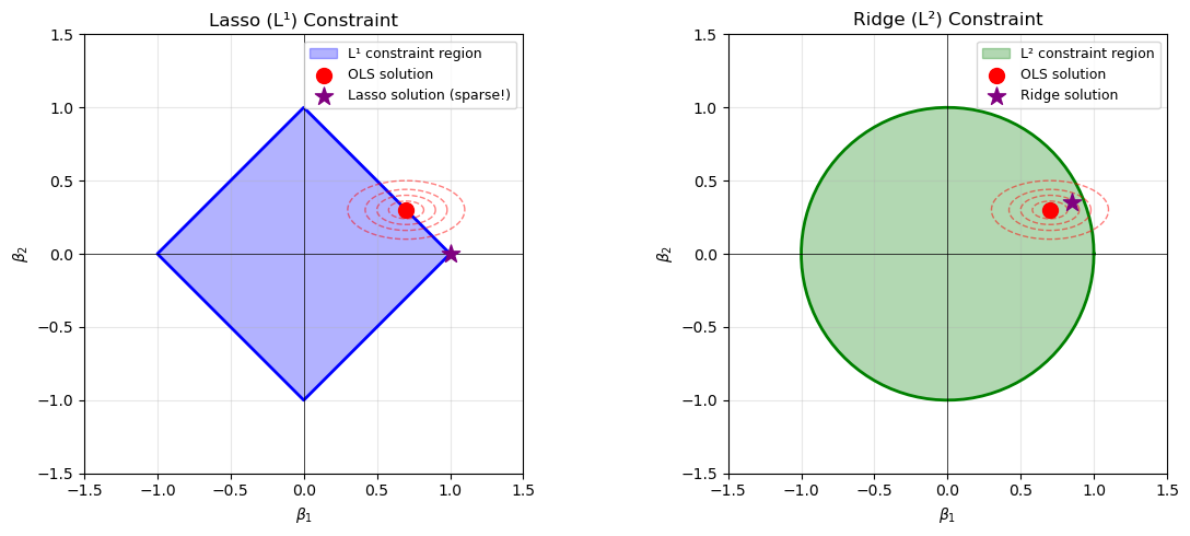
Principal Component Regression (PCR)
Principal Component Regression combines the dimensionality reduction from Notebook 4 with linear regression. The idea is simple:
- Compute the principal components of $X$ (via SVD on centered data).
- Keep only the top $k$ components (those with largest singular values).
- Regress $y$ on these $k$ components.
Linear algebra perspective: We project $X$ onto its best rank-$k$ approximation (in Frobenius norm) and then solve a least-squares problem in the reduced space. This is different from Ridge:
- Ridge shrinks all directions but keeps them.
- PCR discards the smallest singular directions entirely.
PCR is particularly useful when:
- Features are highly correlated (multicollinearity).
- You want interpretable, low-dimensional representations.
- The signal lives in the top principal components while noise dominates the rest.
The trade-off: if the target $y$ is correlated with a small singular direction, PCR will discard useful information.
from sklearn.decomposition import PCA
from sklearn.linear_model import LinearRegression
from sklearn.pipeline import make_pipeline
from sklearn.model_selection import cross_val_score

# Compare PCR with varying number of components
n_components_range = range(1, X_train_scaled.shape[1] + 1)
pcr_scores = []

for n_comp in n_components_range:
    pcr = make_pipeline(
        PCA(n_components=n_comp),
        LinearRegression()
    )
    # Negative MSE (sklearn convention: higher is better)
    scores = cross_val_score(pcr, X_train_scaled, y_train, cv=5, scoring='neg_mean_squared_error')
    pcr_scores.append(-scores.mean())

# Also compute variance explained
pca_full = PCA()
pca_full.fit(X_train_scaled)
var_explained = np.cumsum(pca_full.explained_variance_ratio_)

# Plot
fig, ax1 = plt.subplots(figsize=(10, 5))

ax1.plot(n_components_range, pcr_scores, 'b-o', label='CV MSE')
ax1.set_xlabel('Number of Principal Components')
ax1.set_ylabel('Cross-Validated MSE', color='b')
ax1.tick_params(axis='y', labelcolor='b')

ax2 = ax1.twinx()
ax2.plot(n_components_range, var_explained, 'r--s', label='Variance Explained')
ax2.set_ylabel('Cumulative Variance Explained', color='r')
ax2.tick_params(axis='y', labelcolor='r')
ax2.set_ylim(0, 1.05)

plt.title('Principal Component Regression: Choosing k')
fig.legend(loc='center right', bbox_to_anchor=(0.85, 0.5))
plt.grid(True, alpha=0.3)
plt.tight_layout()
plt.savefig('../images/pcr_components_selection.png')
plt.show()

# Best number of components
best_n_comp = n_components_range[np.argmin(pcr_scores)]
print(f"Best number of components: {best_n_comp}")
print(f"Variance explained: {var_explained[best_n_comp-1]:.2%}")

# Compare with OLS and Ridge
print(f"\nModel Comparison (Test MSE):")
print(f"  OLS (all features):  {test_mse:.4f}")
print(f"  PCR (k={best_n_comp}):       {pcr_scores[best_n_comp-1]:.4f}")
print(f"  Ridge (λ={best_alpha:.2f}):   {test_mse_ridge:.4f}")
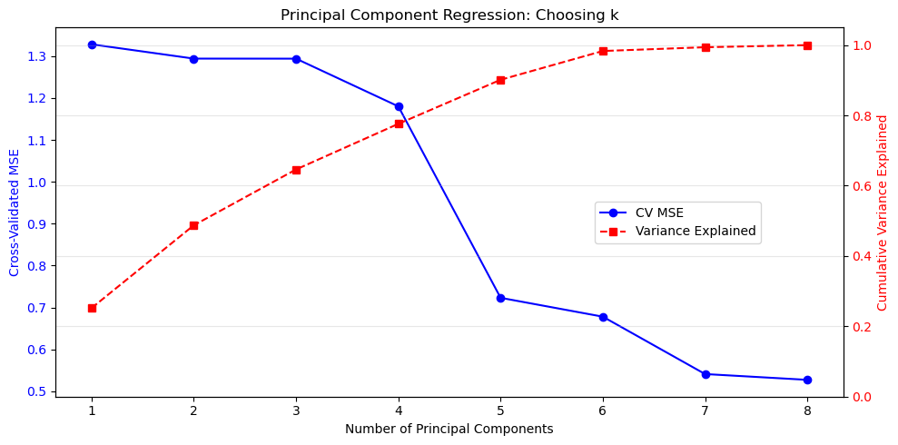
Best number of components: 8
Variance explained: 100.00%

Model Comparison (Test MSE):
  OLS (all features):  0.5381
  PCR (k=8):       0.5272
  Ridge (λ=233.57):   0.4791
Gradient Descent: When the Normal Equations Are Not Enough
For very large datasets, computing $(X^T X)^{-1}$ or even forming $X^T X$ becomes prohibitive. Gradient descent is an iterative optimisation method that uses only first‑order derivatives.
The Linear Algebra of Convergence
The loss function and its gradient:
$$ L(\beta) = \frac{1}{2n}|y - X\beta|_2^2, \qquad \nabla L(\beta) = -\frac{1}{n} X^T (y - X\beta). $$
Starting from $\beta^{(0)}$, we update:
$$ \beta^{(t+1)} = \beta^{(t)} - \eta \nabla L(\beta^{(t)}). $$
Convergence depends on the eigenvalues of $X^T X$. Let $\lambda_{\max}$ and $\lambda_{\min}$ be the largest and smallest eigenvalues. Then:
- The learning rate must satisfy $\eta < \frac{2}{\lambda_{\max}}$ for convergence.
- The convergence rate is governed by the condition number $\kappa = \frac{\lambda_{\max}}{\lambda_{\min}}$.
- When $\kappa$ is large, gradients point in “wrong” directions — the loss surface is a narrow valley.
This is why feature scaling matters: it reduces $\kappa$, making the loss surface more spherical and convergence faster.
# Demonstrate how condition number affects gradient descent convergence
from sklearn.preprocessing import StandardScaler

def gradient_descent_linear(X, y, learning_rate=0.01, n_iter=1000, verbose=False):
    """Batch gradient descent for linear regression."""
    n, p = X.shape
    beta = np.zeros(p)
    losses = []
    for i in range(n_iter):
        residual = y - X @ beta
        grad = - (1/n) * X.T @ residual
        beta -= learning_rate * grad
        loss = (1/(2*n)) * np.linalg.norm(residual)**2
        losses.append(loss)
    return beta, losses

# Use a subset for illustration
X_subset = X_train[:1000]
y_subset = y_train[:1000]

# Add intercept
X_subset_aug = np.hstack([np.ones((X_subset.shape[0], 1)), X_subset])

# Compute eigenvalues of X^T X
eigenvalues = np.linalg.eigvalsh(X_subset_aug.T @ X_subset_aug)
lambda_max, lambda_min = eigenvalues.max(), eigenvalues[eigenvalues > 1e-10].min()
cond_num = lambda_max / lambda_min

print(f"Eigenvalue range: [{lambda_min:.2e}, {lambda_max:.2e}]")
print(f"Condition number: {cond_num:.2e}")
print(f"Max stable learning rate: {2/lambda_max:.2e}")

# Try gradient descent with different learning rates on UNSCALED data
fig, axes = plt.subplots(1, 2, figsize=(14, 5))

# UNSCALED
learning_rates = [1e-10, 1e-9, 1e-8]
for lr in learning_rates:
    _, losses = gradient_descent_linear(X_subset_aug, y_subset, learning_rate=lr, n_iter=200)
    axes[0].plot(losses, label=f'η = {lr:.0e}')
axes[0].set_xlabel('Iteration')
axes[0].set_ylabel('Loss (MSE)')
axes[0].set_title(f'Unscaled Data (κ = {cond_num:.1e})')
axes[0].legend()
axes[0].grid(True, alpha=0.3)
axes[0].set_yscale('log')

# SCALED
scaler = StandardScaler()
X_subset_scaled = scaler.fit_transform(X_subset)
X_subset_scaled_aug = np.hstack([np.ones((X_subset_scaled.shape[0], 1)), X_subset_scaled])

eigenvalues_scaled = np.linalg.eigvalsh(X_subset_scaled_aug.T @ X_subset_scaled_aug)
lambda_max_s, lambda_min_s = eigenvalues_scaled.max(), eigenvalues_scaled[eigenvalues_scaled > 1e-10].min()
cond_num_scaled = lambda_max_s / lambda_min_s

learning_rates_scaled = [0.001, 0.01, 0.1]
for lr in learning_rates_scaled:
    _, losses = gradient_descent_linear(X_subset_scaled_aug, y_subset, learning_rate=lr, n_iter=200)
    axes[1].plot(losses, label=f'η = {lr}')
axes[1].set_xlabel('Iteration')
axes[1].set_ylabel('Loss (MSE)')
axes[1].set_title(f'Scaled Data (κ = {cond_num_scaled:.1f})')
axes[1].legend()
axes[1].grid(True, alpha=0.3)
axes[1].set_yscale('log')

plt.tight_layout()
plt.savefig('../images/gd_condition_number_effect.png')
plt.show()

print(f"\nScaling reduced condition number from {cond_num:.1e} to {cond_num_scaled:.1f}")
print("This allows much larger learning rates and faster convergence.")
Eigenvalue range: [5.59e-02, 3.07e+09]
Condition number: 5.49e+10
Max stable learning rate: 6.52e-10
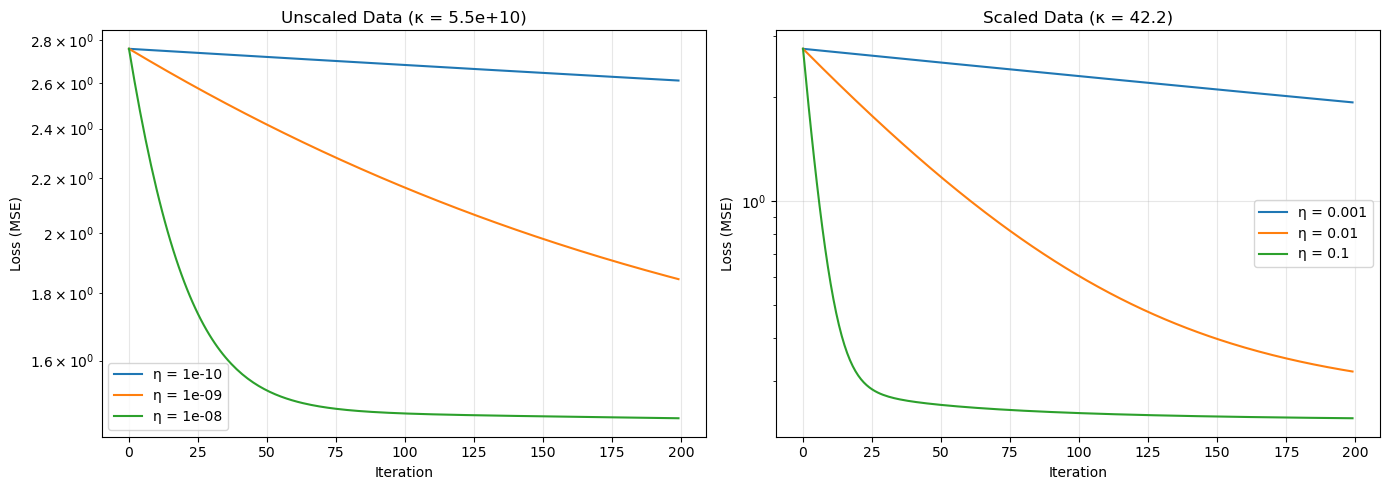
Scaling reduced condition number from 5.5e+10 to 42.2
This allows much larger learning rates and faster convergence.
Let’s apply gradient descent to our housing data.
# Implement batch gradient descent for linear regression on a small subset for illustration
def gradient_descent_linear(X, y, learning_rate=0.01, n_iter=1000, verbose=False):
    n, p = X.shape
    beta = np.zeros(p)
    losses = []
    for i in range(n_iter):
        grad = - (1/n) * X.T @ (y - X @ beta)
        beta -= learning_rate * grad
        loss = (1/(2*n)) * np.linalg.norm(y - X @ beta)**2
        losses.append(loss)
        if verbose and i % 200 == 0:
            print(f"Iter {i}: loss = {loss:.6f}")
    return beta, losses

# Use a small subset for speed
X_small = X_train[:1000]
y_small = y_train[:1000]

# Add intercept column
X_small_aug = np.hstack([np.ones((X_small.shape[0], 1)), X_small])

beta_gd, losses = gradient_descent_linear(X_small_aug, y_small, learning_rate=0.01, n_iter=500)

plt.figure(figsize=(8,4))
plt.plot(losses)
plt.xlabel('Iteration')
plt.ylabel('Loss')
plt.title('Gradient Descent Convergence')
plt.grid(True)
plt.savefig('../images/gradient_descent_convergence_unscaled')
plt.show()

# Compare with closed-form solution on the same subset
beta_closed = np.linalg.lstsq(X_small_aug, y_small, rcond=None)[0]
print(f"Difference between GD and closed-form: {np.linalg.norm(beta_gd - beta_closed):.2e}")
/usr/lib64/python3.14/site-packages/numpy/linalg/_linalg.py:2792: RuntimeWarning: overflow encountered in dot
  sqnorm = x.dot(x)
/tmp/ipykernel_76700/3132444904.py:7: RuntimeWarning: overflow encountered in matmul
  grad = - (1/n) * X.T @ (y - X @ beta)
/tmp/ipykernel_76700/3132444904.py:8: RuntimeWarning: invalid value encountered in subtract
  beta -= learning_rate * grad
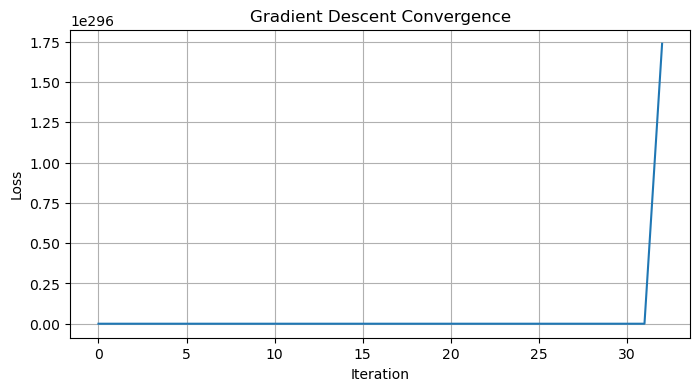
Difference between GD and closed-form: nan
Again, we have scaling issues causing some errors. Large values will dominate gradients, giving rise to instability.
from sklearn.preprocessing import StandardScaler

# 1. Prepare Data
# Use a small subset for speed
X_small = X_train[:1000].copy() # Use .copy() to avoid SettingWithCopyWarning
y_small = y_train[:1000].copy()

# 2. SCALE THE FEATURES (Critical for Gradient Descent!)
scaler = StandardScaler()
X_small_scaled = scaler.fit_transform(X_small)

# Add intercept column AFTER scaling
# (We don't scale the intercept column, it stays as 1s)
X_small_aug = np.hstack([np.ones((X_small_scaled.shape[0], 1)), X_small_scaled])

# 3. Run Gradient Descent
def gradient_descent_linear(X, y, learning_rate=0.01, n_iter=1000, verbose=False):
    n, p = X.shape
    beta = np.zeros(p)
    losses = []
    for i in range(n_iter):
        # Predict
        prediction = X @ beta
        # Residual
        residual = y - prediction
        # Gradient
        grad = - (1/n) * X.T @ residual
        # Update
        beta -= learning_rate * grad

        # Calculate Loss (MSE)
        loss = (1/(2*n)) * np.linalg.norm(residual)**2
        losses.append(loss)

        if verbose and i % 200 == 0:
            print(f"Iter {i}: loss = {loss:.6f}")
    return beta, losses

# With scaled data, learning_rate=0.01 or even 0.1 is usually safe
beta_gd, losses = gradient_descent_linear(X_small_aug, y_small, learning_rate=0.1, n_iter=500, verbose=True)

# Plot convergence
plt.figure(figsize=(8,4))
plt.plot(losses)
plt.xlabel('Iteration')
plt.ylabel('Loss (MSE)')
plt.title('Gradient Descent Convergence (Scaled Data)')
plt.grid(True)
plt.savefig('../images/gradient_descent_convergence_scaled')
plt.show()
Iter 0: loss = 2.758919
Iter 200: loss = 0.234124
Iter 400: loss = 0.230774
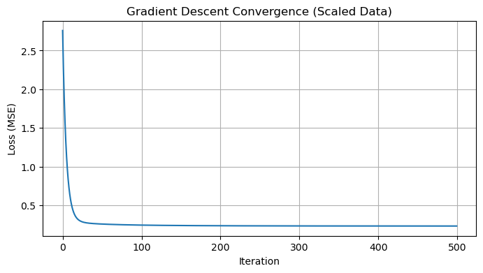
In practice, we use stochastic or mini‑batch gradient descent for large data. sklearn’s SGDRegressor implements these with various loss functions and penalties.
from sklearn.linear_model import SGDRegressor
from sklearn.preprocessing import StandardScaler
from sklearn.pipeline import make_pipeline

# SGDRegressor is sensitive to feature scaling, so we use a pipeline
# penalty=None means no regularization (standard Linear Regression)
sgd_reg = make_pipeline(
    StandardScaler(),
    SGDRegressor(penalty=None, learning_rate='constant', eta0=0.01, max_iter=1000, random_state=42)
)

sgd_reg.fit(X_train, y_train)

# Note: SGDRegressor optimizes a different loss function formulation by default,
# so coefficients might differ slightly from closed-form, but the prediction quality is similar.
print(f"Coefficients: {sgd_reg.named_steps['sgdregressor'].coef_}")
Coefficients: [ 3.97676073e+09 -1.14418633e+10 -1.78357850e+10  1.01065426e+11
 -1.80378121e+10 -3.02815983e+09 -5.43520408e+10 -4.51215845e+10]
Decision Trees and Random Forests
Linear models assume a linear relationship. Decision trees are non‑parametric models that partition the feature space into rectangular regions and assign a constant prediction (or a simple model) in each region. The prediction function is piecewise constant. The basis functions are indicator functions of the leaves. While not linear in the original features, the model is linear in the (high‑dimensional) leaf‑indicator basis.
Random forests combine many decision trees, each trained on a bootstrapped sample and a random subset of features. They reduce variance (overfitting) and often outperform single trees.
When to use trees / forests:
- Nonlinear relationships with interactions.
- When interpretability is desired (a single tree can be visualised).
- When you have mixed categorical and continuous features.
- As a strong baseline before trying deep learning.
from sklearn.tree import DecisionTreeRegressor
from sklearn.ensemble import RandomForestRegressor

# Single decision tree (max depth 10)
tree = DecisionTreeRegressor(max_depth=10, random_state=RANDOM_STATE)
tree.fit(X_train, y_train)
y_test_pred_tree = tree.predict(X_test)
test_mse_tree = mean_squared_error(y_test, y_test_pred_tree)

# Random forest (100 trees)
rf = RandomForestRegressor(n_estimators=100, max_depth=10, random_state=RANDOM_STATE, n_jobs=-1)
rf.fit(X_train, y_train)
y_test_pred_rf = rf.predict(X_test)
test_mse_rf = mean_squared_error(y_test, y_test_pred_rf)

print(f"Decision Tree Test MSE: {test_mse_tree:.4f}")
print(f"Random Forest Test MSE: {test_mse_rf:.4f}")

# Compare with best linear model
print(f"Ridge (poly) Test MSE: {test_mse_ridge:.4f}")
print(f"LassoCV Test MSE:      {test_mse_lasso_cv:.4f}")
Decision Tree Test MSE: 0.3961
Random Forest Test MSE: 0.2752
Ridge (poly) Test MSE: 0.4791
LassoCV Test MSE:      0.5305
Random forests often outperform linear models on complex real‑world data without requiring feature engineering or scaling.
Logistic Regression for Classification
So far we have focused on regression (continuous targets). For binary classification (e.g., spam vs. not spam), logistic regression is a natural extension. It models the probability that an observation belongs to a class using the logistic (sigmoid) function:
$$ P(y=1 \mid x) = \frac{1}{1 + e^{-x^T\beta}}. $$
The decision boundary is linear in the features: $x^T\beta = 0$. The model is fitted by maximum likelihood estimation, which is equivalent to minimising the log‑loss (cross‑entropy). There is no closed‑form solution; we typically use gradient descent or Newton’s method.
We will illustrate logistic regression on a subset of the California housing data by creating a binary target (e.g., whether the median house value is above the median).
from sklearn.linear_model import LogisticRegression
from sklearn.metrics import accuracy_score, classification_report, confusion_matrix

# Create binary target: 1 if house value > median, else 0
# Use the ORIGINAL dataframe to avoid confusion with scaled/transformed versions
y_binary = (df['MedHouseVal'] > df['MedHouseVal'].median()).astype(int).values
X_original = df[feature_names].values  # original features, not overwritten

# Split
X_train_bin, X_test_bin, y_train_bin, y_test_bin = train_test_split(
    X_original, y_binary, test_size=0.2, random_state=RANDOM_STATE
)

# Scale features (important for logistic regression with regularization)
scaler_bin = StandardScaler()
X_train_bin_scaled = scaler_bin.fit_transform(X_train_bin)
X_test_bin_scaled = scaler_bin.transform(X_test_bin)

# Train logistic regression
log_reg = LogisticRegression(max_iter=1000, random_state=RANDOM_STATE)
log_reg.fit(X_train_bin_scaled, y_train_bin)

# Predict
y_pred_bin = log_reg.predict(X_test_bin_scaled)
accuracy = accuracy_score(y_test_bin, y_pred_bin)

print(f"Logistic Regression Accuracy: {accuracy:.4f}")
print("\nClassification Report:")
print(classification_report(y_test_bin, y_pred_bin))

# Coefficients (on scaled features)
coef_df = pd.DataFrame({
    'Feature': feature_names,
    'Coefficient': log_reg.coef_[0]
}).sort_values('Coefficient', key=abs, ascending=False)
print("\nLogistic Regression Coefficients (scaled features):")
print(coef_df)
Logistic Regression Accuracy: 0.8324

Classification Report:
              precision    recall  f1-score   support

           0       0.83      0.84      0.83      2083
           1       0.83      0.83      0.83      2045

    accuracy                           0.83      4128
   macro avg       0.83      0.83      0.83      4128
weighted avg       0.83      0.83      0.83      4128


Logistic Regression Coefficients (scaled features):
      Feature  Coefficient
6    Latitude    -3.532385
7   Longitude    -3.328767
5    AveOccup    -3.094635
0      MedInc     2.512414
3   AveBedrms     0.899888
2    AveRooms    -0.786384
1    HouseAge     0.276838
4  Population     0.062450
Cross‑Validation: A Deeper Look
Cross‑validation (CV) is a technique for assessing how well a model generalises to unseen data. Instead of a single train/validation split, we partition the training data into $k$ folds (typically 5 or 10). For each fold $i$, we train on the other $k-1$ folds and validate on fold $i$. The performance is averaged over the $k$ folds.
# Illustrate 5-fold cross-validation
from sklearn.model_selection import KFold

n_points = 20
X_cv = np.arange(n_points).reshape(-1, 1)
colors = plt.cm.tab10(np.linspace(0, 1, 5))

kf = KFold(n_splits=5, shuffle=True, random_state=3)

fig, axes = plt.subplots(5, 1, figsize=(12, 8))

for i, (train_idx, test_idx) in enumerate(kf.split(X_cv)):
    ax = axes[i]

    # Plot all points
    for j in range(n_points):
        if j in test_idx:
            ax.scatter(j, 0, s=200, c='red', marker='s', label='Test' if j == test_idx[0] else '')
        else:
            ax.scatter(j, 0, s=200, c='blue', marker='o', label='Train' if j == train_idx[0] else '')

    ax.set_xlim(-1, n_points)
    ax.set_ylim(-0.5, 0.5)
    ax.set_yticks([])
    ax.set_ylabel(f'Fold {i+1}', rotation=0, labelpad=30)

    if i == 0:
        ax.legend(loc='upper right', ncol=2)
    if i < 4:
        ax.set_xticks([])

axes[-1].set_xlabel('Sample Index')
axes[2].set_title('5-Fold Cross-Validation', pad=20)

plt.tight_layout()
plt.savefig('../images/cross_validation_illustration.png')
plt.show()
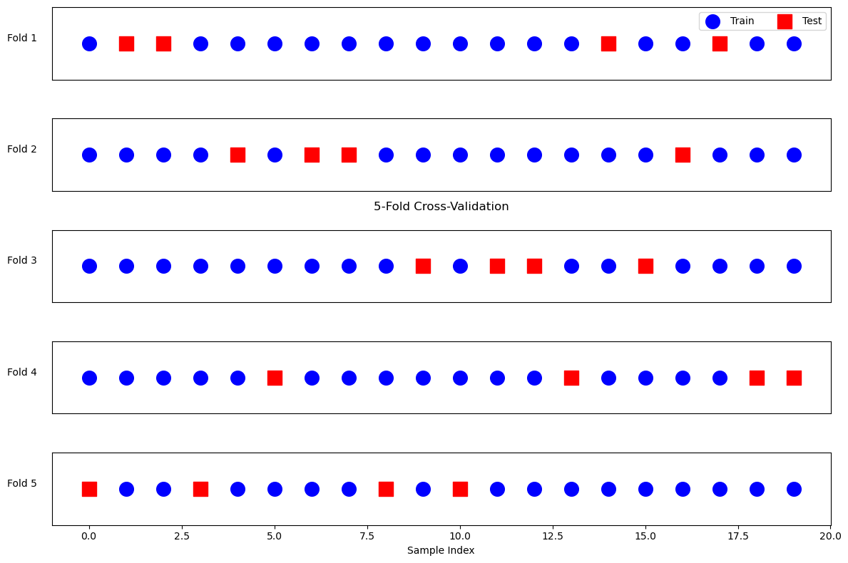
Why cross‑validate? It reduces the variance of the performance estimate and makes better use of limited data. It is also essential for hyperparameter tuning (as we did with Ridge and Lasso).
We already used cross_val_score above. Here’s an explicit example with a linear model on the housing data.
from sklearn.model_selection import cross_val_score, KFold

# 5-fold CV on linear regression
lin_reg_cv = LinearRegression()
scores = cross_val_score(lin_reg_cv, X_train, y_train, cv=5, scoring='r2')
print(f"5-fold CV R² scores: {scores}")
print(f"Mean R²: {scores.mean():.4f} (+/- {scores.std()*2:.4f})")

# We can also use a custom cross-validator
kf = KFold(n_splits=5, shuffle=True, random_state=RANDOM_STATE)
scores_shuffled = cross_val_score(lin_reg_cv, X_train, y_train, cv=kf, scoring='r2')
print(f"Shuffled CV R² scores: {scores_shuffled}")
print(f"Mean R² (shuffled): {scores_shuffled.mean():.4f}")
5-fold CV R² scores: [0.60709214 0.59544452 0.58112984 0.63060861 0.61005689]
Mean R²: 0.6049 (+/- 0.0328)
Shuffled CV R² scores: [0.60563739 0.59602593 0.5917264  0.61941109 0.62268184]
Mean R² (shuffled): 0.6071
Feature Scaling
Many machine learning algorithms are sensitive to the scale of features. For example:
- Gradient descent converges faster when features are on similar scales.
- Regularisation (Ridge, Lasso) penalises coefficients equally; if features have different scales, the penalty is not meaningful.
- Distance‑based methods (k‑nearest neighbours, SVM with RBF kernel) assume all features are comparable.
Linear algebra view: Scaling corresponds to multiplying each column of $X$ by a positive scalar. This changes the condition number and the geometry of the optimisation landscape.
Common scaling techniques:
- Standardisation (Z‑score): $x’ = \frac{x - \mu}{\sigma}$ (mean 0, variance 1).
- Min‑max scaling: $x’ = \frac{x - \min}{\max - \min}$ (range [0,1]).
We should always fit the scaler on the training set and then transform both train and test sets to avoid data leakage.
from sklearn.preprocessing import StandardScaler

# Create scaler
scaler = StandardScaler()

# Fit on training data only
X_train_scaled = scaler.fit_transform(X_train)
X_test_scaled = scaler.transform(X_test)

# Compare condition number before and after scaling
X_train_aug = np.hstack([np.ones((X_train.shape[0], 1)), X_train])
X_train_scaled_aug = np.hstack([np.ones((X_train_scaled.shape[0], 1)), X_train_scaled])

print(f"Condition number (original): {cond(X_train_aug):.2e}")
print(f"Condition number (scaled):   {cond(X_train_scaled_aug):.2e}")

# Fit linear regression on scaled data
lin_reg_scaled = LinearRegression()
lin_reg_scaled.fit(X_train_scaled, y_train)
y_test_pred_scaled = lin_reg_scaled.predict(X_test_scaled)
test_mse_scaled = mean_squared_error(y_test, y_test_pred_scaled)
print(f"Linear regression (scaled) Test MSE: {test_mse_scaled:.4f}")
print(f"Linear regression (original) Test MSE: {test_mse:.4f}")
Condition number (original): 2.40e+05
Condition number (scaled):   6.48e+00
Linear regression (scaled) Test MSE: 0.5381
Linear regression (original) Test MSE: 0.5381
Scaling did not change the linear regression performance because OLS is scale‑invariant (the coefficients adjust accordingly). However, it improves numerical stability and is crucial for regularised models and gradient descent.
Model Interpretation
Interpretability is important in many applications. Different models offer different levels of insight.
Linear Models (Ridge, Lasso)
- Coefficients directly indicate the effect of each feature (assuming features are scaled).
- Sign and magnitude tell us direction and importance.
Decision Trees
- We can visualise the tree structure.
- Feature importance based on how much each feature reduces impurity (e.g., variance for regression, Gini for classification).
Random Forests
- Aggregate feature importance across all trees.
- Can also use SHAP or LIME for local explanations.
Let’s examine coefficients from a scaled linear model and feature importance from a random forest.
# Train Ridge on scaled data (with default alpha)
ridge_scaled = Ridge(alpha=1.0)
ridge_scaled.fit(X_train_scaled, y_train)

# Display coefficients
coef_df = pd.DataFrame({
    'Feature': feature_names,
    'Coefficient': ridge_scaled.coef_
})
print("Ridge coefficients (scaled features):")
print(coef_df.sort_values('Coefficient', key=abs, ascending=False))

# Random forest feature importance
rf.fit(X_train, y_train)  # already fitted earlier, but ensure
importances = rf.feature_importances_
importance_df = pd.DataFrame({
    'Feature': feature_names,
    'Importance': importances
}).sort_values('Importance', ascending=False)

print("\nRandom Forest Feature Importances:")
print(importance_df)

# Plot
plt.figure(figsize=(8,4))
plt.barh(importance_df['Feature'], importance_df['Importance'])
plt.xlabel('Importance')
plt.title('Random Forest Feature Importance')
plt.gca().invert_yaxis()
plt.savefig('../images/RF_feature_importance.png')
plt.show()
Ridge coefficients (scaled features):
      Feature  Coefficient
6    Latitude    -0.896656
7   Longitude    -0.870257
0      MedInc     0.848402
3   AveBedrms     0.332536
2    AveRooms    -0.287161
1    HouseAge     0.125807
5    AveOccup    -0.040522
4  Population    -0.002190

Random Forest Feature Importances:
      Feature  Importance
0      MedInc    0.589486
5    AveOccup    0.137379
6    Latitude    0.078123
7   Longitude    0.077486
1    HouseAge    0.047525
2    AveRooms    0.034377
4  Population    0.018634
3   AveBedrms    0.016990
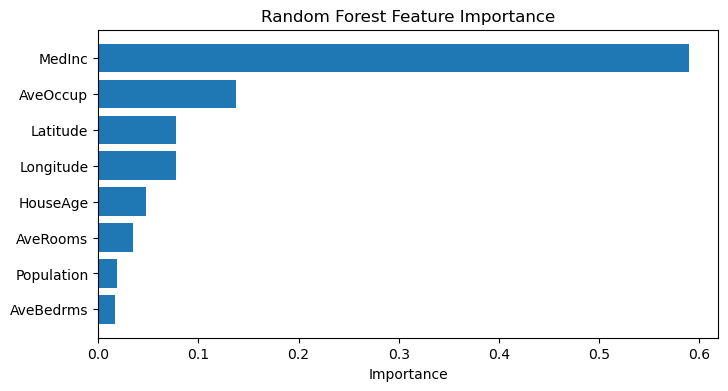
Hyperparameter Tuning with Grid Search
Most models have hyperparameters that are not learned from data (e.g., alpha in Ridge, max_depth in trees, n_estimators in random forests). Tuning them properly is essential for good performance. Choosing hyperparameters is like selecting the optimal basis or regularisation parameter – it changes the solution space.
Grid search exhaustively tries a predefined set of hyperparameter combinations using cross‑validation. sklearn.model_selection.GridSearchCV does this efficiently.
Let’s tune a random forest regressor on the housing data.
from sklearn.model_selection import GridSearchCV

# Define parameter grid
param_grid = {
    'n_estimators': [50, 100],
    'max_depth': [5, 10, None],
    'min_samples_split': [2, 5]
}

# Create random forest
rf_tune = RandomForestRegressor(random_state=42, n_jobs=-1)

# Grid search with 3-fold CV (use a subset of training data for speed)
X_train_subset = X_train[:5000]
y_train_subset = y_train[:5000]

grid_search = GridSearchCV(rf_tune, param_grid, cv=3, scoring='neg_mean_squared_error', verbose=1)
grid_search.fit(X_train_subset, y_train_subset)

print("Best parameters:", grid_search.best_params_)
print("Best CV MSE:", -grid_search.best_score_)

# Evaluate on test set
best_rf = grid_search.best_estimator_
y_test_pred_best_rf = best_rf.predict(X_test)
test_mse_best_rf = mean_squared_error(y_test, y_test_pred_best_rf)
print(f"Tuned Random Forest Test MSE: {test_mse_best_rf:.4f}")
Fitting 3 folds for each of 12 candidates, totalling 36 fits
Best parameters: {'max_depth': None, 'min_samples_split': 2, 'n_estimators': 100}
Best CV MSE: 0.3210370034255883
Tuned Random Forest Test MSE: 0.2928
Summary and Additional Considerations
We have covered a progression of modelling techniques and essential practices:
| Method | Linearity | Regularisation | Feature Selection | Scalability |
|---|---|---|---|---|
| Linear regression | Yes | No | No | Good (closed‑form) |
| Polynomial regression | In features | No | No | Poor (exploding dimension) |
| Ridge | Yes | $L^2$ | No (shrinks only) | Good |
| Lasso | Yes | $L^1$ | Yes | Good (via coordinate descent) |
| Logistic regression | Decision boundary linear | Optional | With L1/L2 | Good |
| Gradient descent | Yes (or any differentiable) | Optional | Optional | Excellent (very large data) |
| Decision trees | No | No (but depth limits) | Implicitly | Moderate |
| Random forests | No | No (ensemble reduces variance) | Implicitly | Moderate (parallelisable) |
Bias–variance trade-off: Simple models (linear) have high bias but low variance. Complex models (deep trees) have low bias but high variance. Regularisation and ensembles (random forests) try to balance this.
What else could be added?
- Support vector machines (SVM) – geometric margin classifiers.
- Neural networks – highly flexible nonlinear models.
- Time series models (ARIMA, etc.).
- Model selection criteria (AIC, BIC).
Bibliography
Mathematics
- Gene H. Golub and Charles F. Van Loan, Matrix Computations. Johns Hopkins University Press, 2013.
- Mark H. Holmes, Introduction to scientific computing and data analysis. Vol. 13. Springer Nature, 2023.
- David C. Lay, Steven R. Lay, and Judith J. McDonald, Linear Algebra and Its Applications, Pearson, 2021. ISBN 013588280X.
- https://ubcmath.github.io/MATH307/index.html
- https://eecs16b.org/notes/fa23/note16.pdf
- https://en.wikipedia.org/wiki/Low-rank_approximation
- https://www-labs.iro.umontreal.ca/~grabus/courses/ift6760_W20_files/lecture-5.pdf
- https://www.statology.org/polynomial-regression-python/
- https://en.wikipedia.org/wiki/Mean_squared_error
- https://en.wikipedia.org/wiki/Peak_signal-to-noise_ratio
Modelling
- https://www.geeksforgeeks.org/machine-learning/what-is-ridge-regression/
- https://www.geeksforgeeks.org/machine-learning/what-is-lasso-regression/
- https://www.geeksforgeeks.org/machine-learning/principal-component-regression-pcr/
- https://www.geeksforgeeks.org/machine-learning/gradient-descent-algorithm-and-its-variants/
- https://www.geeksforgeeks.org/machine-learning/decision-tree/
- https://www.geeksforgeeks.org/machine-learning/random-forest-algorithm-in-machine-learning/
Python
NumPy (https://numpy.org/doc/stable/index.html)
- numpy basics: https://numpy.org/doc/stable/user/absolute_beginners.html
- numpy.array: https://numpy.org/doc/stable/reference/generated/numpy.array.html
- numpy.hstack: https://numpy.org/doc/stable/reference/generated/numpy.hstack.html (Stack arrays in sequence horizontally (column wise).)
- numpy.column_stack: https://numpy.org/doc/stable/reference/generated/numpy.column_stack.html (Stack 1-D arrays as columns into a 2-D array.)
- numpy.shape: https://numpy.org/doc/stable/reference/generated/numpy.shape.html (Return the shape of an array.)
- numpy.polyfit: https://numpy.org/doc/stable/reference/generated/numpy.polyfit.html (Least squares polynomial fit.)
- numpy.mean: https://numpy.org/doc/stable/reference/generated/numpy.mean.html (Compute the arithmetic mean along the specified axis.)
- numpy.poly1d: https://numpy.org/doc/stable/reference/generated/numpy.poly1d.html (A one-dimensional polynomial class.)
- numpy.set_printoptions: https://numpy.org/doc/stable/reference/generated/numpy.set_printoptions.html (These options determine the way floating point numbers, arrays and other NumPy objects are displayed.)
- numpy.finfo: https://numpy.org/doc/stable/reference/generated/numpy.finfo.html (Machine limits for floating point types.)
- numpy.logspace: https://numpy.org/doc/stable/reference/generated/numpy.logspace.html (Return numbers spaced evenly on a log scale.)
- numpy.sum: https://numpy.org/doc/stable/reference/generated/numpy.sum.html (Sum of array elements over a given axis.)
- numpy.abs: https://numpy.org/doc/stable/reference/generated/numpy.absolute.html (Calculate the absolute value element-wise.)
- numpy.ndarray.T: https://numpy.org/doc/stable/reference/generated/numpy.ndarray.T.html (View of the transposed array.)
- numpy.ones: https://numpy.org/doc/stable/reference/generated/numpy.ones.html (Return a new array of given shape and type, filled with ones.)
- numpy.zeros: https://numpy.org/doc/stable/reference/generated/numpy.zeros.html (Return a new array of given shape and type, filled with zeros.)
- numpy.diag: https://numpy.org/doc/stable/reference/generated/numpy.diag.html (Extract a diagonal or construct a diagonal array.)
- numpy.cumsum: https://numpy.org/doc/stable/reference/generated/numpy.cumsum.html (Return the cumulative sum of the elements along a given axis.)
- numpy.meshgrid: https://numpy.org/doc/stable/reference/generated/numpy.meshgrid.html (Return a tuple of coordinate matrices from coordinate vectors.)
- numpy.linspace: https://numpy.org/doc/stable/reference/generated/numpy.linspace.html (Return evenly spaced numbers over a specified interval.)
- numpy.ravel: https://numpy.org/doc/stable/reference/generated/numpy.ravel.html (Return a contiguous flattened array.)
- numpy.vstack: https://numpy.org/doc/stable/reference/generated/numpy.vstack.html (Stack arrays in sequence vertically (row wise).)
numpy.random (https://numpy.org/doc/stable/reference/random/index.html)
- numpy.random.seed: https://numpy.org/doc/stable/reference/random/generated/numpy.random.seed.html (Reseed the singleton RandomState instance.)
- numpy.random.normal: https://numpy.org/doc/stable/reference/random/generated/numpy.random.normal.html (Draw random samples from a normal (Gaussian) distribution.)
- numpy.random.default_rng: https://numpy.org/doc/stable/reference/random/generator.html (Construct a new Generator with the default BitGenerator (PCG64).)
- numpy.random.uniform: https://numpy.org/doc/stable/reference/random/generated/numpy.random.uniform.html (Draw samples from a uniform distribution.)
numpy.linalg (https://numpy.org/doc/stable/reference/routines.linalg.html)
- numpy.linalg.qr: https://numpy.org/doc/stable/reference/generated/numpy.linalg.qr.html (Compute the QR factorization of a matrix.)
- numpy.linalg.svd: https://numpy.org/doc/stable/reference/generated/numpy.linalg.svd.html (Singular Value Decomposition.)
- numpy.linalg.solve: https://numpy.org/doc/stable/reference/generated/numpy.linalg.solve.html (Solve a linear matrix equation, or system of linear scalar equations.)
- numpy.linalg.lstsq: https://numpy.org/doc/stable/reference/generated/numpy.linalg.lstsq.html (Return the least-squares solution to a linear matrix equation.)
- numpy.linalg.norm: https://numpy.org/doc/stable/reference/generated/numpy.linalg.norm.html (Matrix or vector norm.)
- numpy.linalg.pinv: https://numpy.org/doc/stable/reference/generated/numpy.linalg.pinv.html (Compute the (Moore-Penrose) pseudo-inverse of a matrix.)
- numpy.linalg.cond: https://numpy.org/doc/stable/reference/generated/numpy.linalg.cond.html (Compute the condition number of a matrix.)
Matplotlib (https://matplotlib.org/stable/users/getting_started/)
- matplotlib.pyplot: https://matplotlib.org/stable/api/pyplot_summary.html
- matplotlib.figure: https://matplotlib.org/stable/api/figure_api.html (Implements the following classes:
FigureandSubFigure) - mpl_toolkits.mplot3d.axes3d.Axes3D.plot_surface: https://matplotlib.org/stable/api/_as_gen/mpl_toolkits.mplot3d.axes3d.Axes3D.plot_surface.html#mpl_toolkits.mplot3d.axes3d.Axes3D.plot_surface (Create a surface plot.)
- colormaps: https://matplotlib.org/stable/users/explain/colors/colormaps.html
matplotlib.pyplot
- matplotlib.pyplot.plot: https://matplotlib.org/stable/api/_as_gen/matplotlib.pyplot.plot.html (Plot y versus x as lines and/or markers.)
- matplotlib.pyplot.quiver: https://matplotlib.org/stable/api/_as_gen/matplotlib.pyplot.quiver.html (Plot a 2D field of arrows.)
- matplotlib.pyplot.tight_layout: https://matplotlib.org/stable/api/_as_gen/matplotlib.pyplot.tight_layout.html (Adjust the padding between and around subplots.)
- matplotlib.pyplot.legend: https://matplotlib.org/stable/api/_as_gen/matplotlib.pyplot.legend.html (Place a legend on the Axes.)
- matplotlib.pyplot.show: https://matplotlib.org/stable/api/_as_gen/matplotlib.pyplot.show.html (Display all open figures.)
- matplotlib.pyplot.xlabel: https://matplotlib.org/stable/api/_as_gen/matplotlib.pyplot.xlabel.html (Set the label for the x-axis.)
- matplotlib.pyplot.ylabel: https://matplotlib.org/stable/api/_as_gen/matplotlib.pyplot.ylabel.html (Set the label for the y-axis.)
- matplotlib.pyplot.title: https://matplotlib.org/stable/api/_as_gen/matplotlib.pyplot.title.html (Set a title for the Axes.)
- matplotlib.pyplot.scatter: https://matplotlib.org/stable/api/_as_gen/matplotlib.pyplot.scatter.html (A scatter plot of y vs. x with varying marker size and/or color.)
- matplotlib.pyplot.imshow: https://matplotlib.org/stable/api/_as_gen/matplotlib.pyplot.imshow.html (Display data as an image, i.e., on a 2D regular raster.)
- matplotlib.pyplot.axis: https://matplotlib.org/stable/api/_as_gen/matplotlib.pyplot.axis.html (Convenience method to get or set some axis properties.)
- matplotlib.pyplot.semilogy: https://matplotlib.org/stable/api/_as_gen/matplotlib.pyplot.semilogy.html (Make a plot with log scaling on the y-axis.)
- matplotlib.pyplot.subplots: https://matplotlib.org/stable/api/_as_gen/matplotlib.pyplot.subplots.html (Create a figure and a set of subplots.)
- matplotlib.pyplot.contour: https://matplotlib.org/stable/api/_as_gen/matplotlib.pyplot.contour.html (Plot contour lines.)
- matplotlib.pyplot.contourf: https://matplotlib.org/stable/api/_as_gen/matplotlib.pyplot.contourf.html (Plot filled contours.)
- matplotlib.pyplot.axhline: https://matplotlib.org/stable/api/_as_gen/matplotlib.pyplot.axhline.html (Add a horizontal line spanning the whole or fraction of the Axes.)
- matplotlib.pyplot.axvline: https://matplotlib.org/stable/api/_as_gen/matplotlib.pyplot.axvline.html (Add a vertical line spanning the whole or fraction of the Axes.)
- matplotlib.pyplot.gca: https://matplotlib.org/stable/api/_as_gen/matplotlib.pyplot.gca.html (Get the current Axes.)
matplotlib.figure
- matplotlib.figure.Figure.add_subplot : https://matplotlib.org/stable/api/_as_gen/matplotlib.figure.Figure.add_subplot.html (Add an
Axesto the figure as part of a subplot arrangement.)]
matplotlib.axes
- matplotlib.axes.Axes.set_title: https://matplotlib.org/stable/api/_as_gen/matplotlib.axes.Axes.set_title.html (Set a title for the Axes.)
- matplotlib.axes.Axes.imshow: https://matplotlib.org/stable/api/_as_gen/matplotlib.axes.Axes.imshow.html (Display data as an image, i.e., on a 2D regular raster.)
- matplotlib.axes.Axes.axis: https://matplotlib.org/stable/api/_as_gen/matplotlib.axes.Axes.axis.html (Convenience method to get or set some axis properties.)
- matplotlib.axes.Axes.text: https://matplotlib.org/stable/api/_as_gen/matplotlib.axes.Axes.text.html (Add text to the Axes.)
- matplotlib.axes.Axes.set_xlabel: https://matplotlib.org/stable/api/_as_gen/matplotlib.axes.Axes.set_xlabel.html (Set the label for the x-axis.)
- matplotlib.axes.Axes.set_ylabel: https://matplotlib.org/stable/api/_as_gen/matplotlib.axes.Axes.set_ylabel.html (Set the label for the y-axis.)
- matplotlib.axes.Axes.set_xlim: https://matplotlib.org/stable/api/_as_gen/matplotlib.axes.Axes.set_xlim.html (Set the x-axis view limits.)
- matplotlib.axes.Axes.set_aspect: https://matplotlib.org/stable/api/_as_gen/matplotlib.axes.Axes.set_aspect.html (Set the aspect ratio of the Axes scaling, i.e. y/x-scale.)
Scatter plots with line of best fit
- https://stackoverflow.com/questions/37234163/how-to-add-a-line-of-best-fit-to-scatter-plot
- https://www.statology.org/line-of-best-fit-python/
- https://stackoverflow.com/questions/6148207/linear-regression-with-matplotlib-numpy
Pandas
- pandas basics: https://pandas.pydata.org/docs/user_guide/index.html
- pandas.DataFrame: https://pandas.pydata.org/pandas-docs/stable/reference/api/pandas.DataFrame.html (Two-dimensional, size-mutable, potentially heterogeneous tabular data.)
pandas.DataFrame
- pandas.DataFrame.describe: https://pandas.pydata.org/pandas-docs/stable/reference/api/pandas.DataFrame.describe.html (Generate descriptive statistics.)
- pandas.DataFrame.corr: https://pandas.pydata.org/pandas-docs/stable/reference/api/pandas.DataFrame.corr.html (Compute pairwise correlation of columns, excluding NA/null values.)
- pandas.DataFrame.to_numpy: https://pandas.pydata.org/docs/reference/api/pandas.DataFrame.to_numpy.html (Convert the DataFrame to a NumPy array.)
- pandas.DataFrame.plot: https://pandas.pydata.org/pandas-docs/stable/reference/api/pandas.DataFrame.plot.html (Make plots of Series or DataFrame.)
scikit-learn
- sklearn basis: https://scikit-learn.org/stable/getting_started.html#fitting-and-predicting-estimator-basics
- sklearn.datasets.fetch_california_housing: https://scikit-learn.org/stable/modules/generated/sklearn.datasets.fetch_california_housing.html (Load the California housing dataset (regression).)
- sklearn.tree.DecisionTreeRegressor: https://scikit-learn.org/stable/modules/generated/sklearn.tree.DecisionTreeRegressor.html (A decision tree regressor.)
- sklearn.ensemble.RandomForestRegressor: https://scikit-learn.org/stable/modules/generated/sklearn.ensemble.RandomForestRegressor.html (A random forest regressor.)
- sklearn.pipeline.make_pipeline: https://scikit-learn.org/stable/modules/generated/sklearn.pipeline.make_pipeline.html (Construct a Pipeline from the given estimators.)
- sklearn.decomposition.PCA: https://scikit-learn.org/stable/modules/generated/sklearn.decomposition.PCA.html (Principal component analysis (PCA).)
sklearn.preprocessing
- sklearn.preprocessing.PolynomialFeatures: https://scikit-learn.org/stable/modules/generated/sklearn.preprocessing.PolynomialFeatures.html (Generate polynomial and interaction features.)
- sklearn.preprocessing: https://scikit-learn.org/stable/modules/generated/sklearn.preprocessing.StandardScaler.html (Standardize features by removing the mean and scaling to unit variance.)
sklearn.linear_model
- sklearn.linear_model.LinearRegression: https://scikit-learn.org/stable/modules/generated/sklearn.linear_model.LinearRegression.html (Ordinary least squares Linear Regression.)
- sklearn.linear_model.Ridge: https://scikit-learn.org/stable/modules/generated/sklearn.linear_model.Ridge.html (Linear least squares with l2 regularization.)
- sklearn.linear_model.Lasso: https://scikit-learn.org/stable/modules/generated/sklearn.linear_model.Lasso.html (Linear Model trained with L1 prior as regularizer (aka the Lasso).)
- sklearn.linear_model.LassoCV: https://scikit-learn.org/stable/modules/generated/sklearn.linear_model.LassoCV.html (Lasso linear model with iterative fitting along a regularization path.)
- sklearn.linear_model.SGDRegressor: https://scikit-learn.org/stable/modules/generated/sklearn.linear_model.SGDRegressor.html (Linear model fitted by minimizing a regularized empirical loss with SGD.)
sklearn.model_selection
- sklearn.model_selection.train_test_split: https://scikit-learn.org/stable/modules/generated/sklearn.model_selection.train_test_split.html (Split arrays or matrices into random train and test subsets.)
- sklearn.model_selection.cross_val_score: https://scikit-learn.org/stable/modules/generated/sklearn.model_selection.cross_val_score.html (Evaluate a score by cross-validation.)
- sklearn.model_selection.KFold: https://scikit-learn.org/stable/modules/generated/sklearn.model_selection.KFold.html (K-Fold cross-validator.)
sklearn.metrics
- sklearn.metrics.mean_squared_error: https://scikit-learn.org/stable/modules/generated/sklearn.metrics.mean_squared_error.html (Mean squared error regression loss.)
- sklearn.metrics.r2_score: https://scikit-learn.org/stable/modules/generated/sklearn.metrics.r2_score.html (R^2 (coefficient of determination) regression score function.)
Pillow
- PIL basics: https://pillow.readthedocs.io/en/stable/
- PIL.Image: https://pillow.readthedocs.io/en/stable/reference/Image.html
Math
- Math basics: https://docs.python.org/3/library/math.html
- math.ceil: https://docs.python.org/3/library/math.html#math.ceil (Return the ceiling of x, the smallest integer greater than or equal to x)
License
This project is licensed under the MIT License. See the LICENSE file for details.